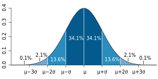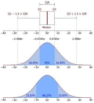
In probability theory and statistics, the cumulative distribution function (CDF) of a real-valued random variable , or just distribution function of , evaluated at , is the probability that will take a value less than or equal to .

In probability theory, the expected value is a generalization of the weighted average. Informally, the expected value is the mean of the possible values a random variable can take, weighted by the probability of those outcomes. Since it is obtained through arithmetic, the expected value sometimes may not even be included in the sample data set; it is not the value you would "expect" to get in reality.

Probability theory or probability calculus is the branch of mathematics concerned with probability. Although there are several different probability interpretations, probability theory treats the concept in a rigorous mathematical manner by expressing it through a set of axioms. Typically these axioms formalise probability in terms of a probability space, which assigns a measure taking values between 0 and 1, termed the probability measure, to a set of outcomes called the sample space. Any specified subset of the sample space is called an event.

In probability theory and statistics, a probability distribution is the mathematical function that gives the probabilities of occurrence of possible outcomes for an experiment. It is a mathematical description of a random phenomenon in terms of its sample space and the probabilities of events.

A random variable is a mathematical formalization of a quantity or object which depends on random events. The term 'random variable' in its mathematical definition refers to neither randomness nor variability but instead is a mathematical function in which

In probability theory, a probability density function (PDF), density function, or density of an absolutely continuous random variable, is a function whose value at any given sample in the sample space can be interpreted as providing a relative likelihood that the value of the random variable would be equal to that sample. Probability density is the probability per unit length, in other words, while the absolute likelihood for a continuous random variable to take on any particular value is 0, the value of the PDF at two different samples can be used to infer, in any particular draw of the random variable, how much more likely it is that the random variable would be close to one sample compared to the other sample.

In probability, and statistics, a multivariate random variable or random vector is a list or vector of mathematical variables each of whose value is unknown, either because the value has not yet occurred or because there is imperfect knowledge of its value. The individual variables in a random vector are grouped together because they are all part of a single mathematical system — often they represent different properties of an individual statistical unit. For example, while a given person has a specific age, height and weight, the representation of these features of an unspecified person from within a group would be a random vector. Normally each element of a random vector is a real number.
In probability theory, there exist several different notions of convergence of sequences of random variables, including convergence in probability, convergence in distribution, and almost sure convergence. The different notions of convergence capture different properties about the sequence, with some notions of convergence being stronger than others. For example, convergence in distribution tells us about the limit distribution of a sequence of random variables. This is a weaker notion than convergence in probability, which tells us about the value a random variable will take, rather than just the distribution.

In probability and statistics, a Bernoulli process is a finite or infinite sequence of binary random variables, so it is a discrete-time stochastic process that takes only two values, canonically 0 and 1. The component Bernoulli variablesXi are identically distributed and independent. Prosaically, a Bernoulli process is a repeated coin flipping, possibly with an unfair coin. Every variable Xi in the sequence is associated with a Bernoulli trial or experiment. They all have the same Bernoulli distribution. Much of what can be said about the Bernoulli process can also be generalized to more than two outcomes ; this generalization is known as the Bernoulli scheme.

In probability theory, the law of large numbers (LLN) is a mathematical law that states that the average of the results obtained from a large number of independent random samples converges to the true value, if it exists. More formally, the LLN states that given a sample of independent and identically distributed values, the sample mean converges to the true mean.
In probability theory and statistics, the conditional probability distribution is a probability distribution that describes the probability of an outcome given the occurrence of a particular event. Given two jointly distributed random variables and , the conditional probability distribution of given is the probability distribution of when is known to be a particular value; in some cases the conditional probabilities may be expressed as functions containing the unspecified value of as a parameter. When both and are categorical variables, a conditional probability table is typically used to represent the conditional probability. The conditional distribution contrasts with the marginal distribution of a random variable, which is its distribution without reference to the value of the other variable.
In information theory, the information content, self-information, surprisal, or Shannon information is a basic quantity derived from the probability of a particular event occurring from a random variable. It can be thought of as an alternative way of expressing probability, much like odds or log-odds, but which has particular mathematical advantages in the setting of information theory.

In probability and statistics, the Dirichlet distribution, often denoted , is a family of continuous multivariate probability distributions parameterized by a vector of positive reals. It is a multivariate generalization of the beta distribution, hence its alternative name of multivariate beta distribution (MBD). Dirichlet distributions are commonly used as prior distributions in Bayesian statistics, and in fact, the Dirichlet distribution is the conjugate prior of the categorical distribution and multinomial distribution.
Probability theory and statistics have some commonly used conventions, in addition to standard mathematical notation and mathematical symbols.

In probability theory and statistics, the characteristic function of any real-valued random variable completely defines its probability distribution. If a random variable admits a probability density function, then the characteristic function is the Fourier transform of the probability density function. Thus it provides an alternative route to analytical results compared with working directly with probability density functions or cumulative distribution functions. There are particularly simple results for the characteristic functions of distributions defined by the weighted sums of random variables.
In probability theory, random element is a generalization of the concept of random variable to more complicated spaces than the simple real line. The concept was introduced by Maurice Fréchet who commented that the “development of probability theory and expansion of area of its applications have led to necessity to pass from schemes where (random) outcomes of experiments can be described by number or a finite set of numbers, to schemes where outcomes of experiments represent, for example, vectors, functions, processes, fields, series, transformations, and also sets or collections of sets.”
In probability theory and statistics, the Dirichlet-multinomial distribution is a family of discrete multivariate probability distributions on a finite support of non-negative integers. It is also called the Dirichlet compound multinomial distribution (DCM) or multivariate Pólya distribution. It is a compound probability distribution, where a probability vector p is drawn from a Dirichlet distribution with parameter vector , and an observation drawn from a multinomial distribution with probability vector p and number of trials n. The Dirichlet parameter vector captures the prior belief about the situation and can be seen as a pseudocount: observations of each outcome that occur before the actual data is collected. The compounding corresponds to a Pólya urn scheme. It is frequently encountered in Bayesian statistics, machine learning, empirical Bayes methods and classical statistics as an overdispersed multinomial distribution.
In probability theory and statistical mechanics, the Gaussian free field (GFF) is a Gaussian random field, a central model of random surfaces.
In mathematics, Anderson's theorem is a result in real analysis and geometry which says that the integral of an integrable, symmetric, unimodal, non-negative function f over an n-dimensional convex body K does not decrease if K is translated inwards towards the origin. This is a natural statement, since the graph of f can be thought of as a hill with a single peak over the origin; however, for n ≥ 2, the proof is not entirely obvious, as there may be points x of the body K where the value f(x) is larger than at the corresponding translate of x.
In probability theory and statistics, an inverse distribution is the distribution of the reciprocal of a random variable. Inverse distributions arise in particular in the Bayesian context of prior distributions and posterior distributions for scale parameters. In the algebra of random variables, inverse distributions are special cases of the class of ratio distributions, in which the numerator random variable has a degenerate distribution.


