Cumulative frequency distribution, adapted cumulative probability distribution, and confidence intervals
Cumulative frequency analysis is the analysis of the frequency of occurrence of values of a phenomenon less than a reference value. The phenomenon may be time- or space-dependent. Cumulative frequency is also called frequency of non-exceedance.
Cumulative frequency analysis is performed to obtain insight into how often a certain phenomenon (feature) is below a certain value. This may help in describing or explaining a situation in which the phenomenon is involved, or in planning interventions, for example in flood protection.[1]
This statistical technique can be used to see how likely an event like a flood is going to happen again in a certain time frame in the future, based on how often it happened in the past. It can be adapted to bring in things like climate change causing wetter winters and drier summers.
Principles
Definitions
Frequency analysis[2] is the analysis of how often, or how frequently, an observed phenomenon occurs in a certain range.
Frequency analysis applies to a record of length N of observed data X1, X2, X3 . . . XN on a variable phenomenon X. The record may be time-dependent (e.g. rainfall measured in one spot) or space-dependent (e.g. crop yields in an area) or otherwise.
The cumulative frequencyMXr of a reference value Xr is the frequency by which the observed values X are less than or equal to Xr.
The relative cumulative frequencyFc can be calculated from:
Fc = MXr / N
where N is the number of data
Briefly this expression can be noted as:
Fc = M / N
When Xr = Xmin, where Xmin is the unique minimum value observed, it is found that Fc = 1/N, because M = 1. On the other hand, when Xr = Xmax, where Xmax is the unique maximum value observed, it is found that Fc = 1, because M = N. Hence, when Fc = 1 this signifies that Xr is a value whereby all data are less than or equal to Xr.
In percentage the equation reads:
Fc (%) = 100 M / N
Probability estimate
From cumulative frequency
The cumulative probabilityPc of X to be smaller than or equal to Xr can be estimated in several ways on the basis of the cumulative frequency M.
One way is to use the relative cumulative frequency Fc as an estimate.
Another way is to take into account the possibility that in rare cases X may assume values larger than the observed maximum Xmax. This can be done dividing the cumulative frequency M by N+1 instead of N. The estimate then becomes:
Pc = M / (N+1)
There exist also other proposals for the denominator (see plotting positions).
By ranking technique
Ranked cumulative probabilities
The estimation of probability is made easier by ranking the data.
When the observed data of X are arranged in ascending order (X1 ≤ X2 ≤ X3 ≤ ⋯ ≤ XN, the minimum first and the maximum last), and Ri is the rank number of the observation Xi, where the adfix i indicates the serial number in the range of ascending data, then the cumulative probability may be estimated by:
Pc = Ri / (N + 1)
When, on the other hand, the observed data from X are arranged in descending order, the maximum first and the minimum last, and Rj is the rank number of the observation Xj, the cumulative probability may be estimated by:
Pc = 1 − Rj / (N + 1)
Fitting of probability distributions
Continuous distributions
Different cumulative normal probability distributions with their parameters
To present the cumulative frequency distribution as a continuous mathematical equation instead of a discrete set of data, one may try to fit the cumulative frequency distribution to a known cumulative probability distribution,.[2][3] If successful, the known equation is enough to report the frequency distribution and a table of data will not be required. Further, the equation helps interpolation and extrapolation. However, care should be taken with extrapolating a cumulative frequency distribution, because this may be a source of errors. One possible error is that the frequency distribution does not follow the selected probability distribution any more beyond the range of the observed data.
Any equation that gives the value 1 when integrated from a lower limit to an upper limit agreeing well with the data range, can be used as a probability distribution for fitting. A sample of probability distributions that may be used can be found in probability distributions.
Probability distributions can be fitted by several methods,[2] for example:
the regression method, linearizing the probability distribution through transformation and determining the parameters from a linear regression of the transformed Pc (obtained from ranking) on the transformed X data.
Application of both types of methods using for example
often shows that a number of distributions fit the data well and do not yield significantly different results, while the differences between them may be small compared to the width of the confidence interval.[2] This illustrates that it may be difficult to determine which distribution gives better results. For example, approximately normally distributed data sets can be fitted to a large number of different probability distributions.[4] while negatively skewed distributions can be fitted to square normal and mirrored Gumbel distributions.[5]
Cumulative frequency distribution with a discontinuity
Discontinuous distributions
Sometimes it is possible to fit one type of probability distribution to the lower part of the data range and another type to the higher part, separated by a breakpoint, whereby the overall fit is improved.
The figure gives an example of a useful introduction of such a discontinuous distribution for rainfall data in northern Peru, where the climate is subject to the behavior Pacific Ocean current El Niño. When the Niño extends to the south of Ecuador and enters the ocean along the coast of Peru, the climate in Northern Peru becomes tropical and wet. When the Niño does not reach Peru, the climate is semi-arid. For this reason, the higher rainfalls follow a different frequency distribution than the lower rainfalls.[6]
Prediction
Uncertainty
When a cumulative frequency distribution is derived from a record of data, it can be questioned if it can be used for predictions.[7] For example, given a distribution of river discharges for the years 1950–2000, can this distribution be used to predict how often a certain river discharge will be exceeded in the years 2000–50? The answer is yes, provided that the environmental conditions do not change. If the environmental conditions do change, such as alterations in the infrastructure of the river's watershed or in the rainfall pattern due to climatic changes, the prediction on the basis of the historical record is subject to a systematic error. Even when there is no systematic error, there may be a random error, because by chance the observed discharges during 1950–2000 may have been higher or lower than normal, while on the other hand the discharges from 2000 to 2050 may by chance be lower or higher than normal. Issues around this have been explored in the book The Black Swan.
Confidence intervals
Binomial distributions for Pc = 0.1 (blue), 0.5 (green) and 0.8 (red) in a sample of size N = 20. The distribution is symmetrical only when Pc = 0.590% binomial confidence belts on a log scale.
Probability theory can help to estimate the range in which the random error may be. In the case of cumulative frequency there are only two possibilities: a certain reference value X is exceeded or it is not exceeded. The sum of frequency of exceedance and cumulative frequency is 1 or 100%. Therefore, the binomial distribution can be used in estimating the range of the random error.
According to the normal theory, the binomial distribution can be approximated and for large N standard deviation Sd can be calculated as follows:
Sd =√Pc(1 − Pc)/N
where Pc is the cumulative probability and N is the number of data. It is seen that the standard deviation Sd reduces at an increasing number of observations N.
The determination of the confidence interval of Pc makes use of Student's t-test (t). The value of t depends on the number of data and the confidence level of the estimate of the confidence interval. Then, the lower (L) and upper (U) confidence limits of Pc in a symmetrical distribution are found from:
L = Pc − t⋅Sd
U = Pc + t⋅Sd
This is known as Wald interval.[8] However, the binomial distribution is only symmetrical around the mean when Pc = 0.5, but it becomes asymmetrical and more and more skew when Pc approaches 0 or 1. Therefore, by approximation, Pc and 1−Pc can be used as weight factors in the assignation of t.Sd to L and U:
L = Pc − 2⋅Pc⋅t⋅Sd
U = Pc + 2⋅(1−Pc)⋅t⋅Sd
where it can be seen that these expressions for Pc = 0.5 are the same as the previous ones.
Example
N = 25, Pc = 0.8, Sd = 0.08, confidence level is 90%, t = 1.71, L = 0.58, U = 0.85 Thus, with 90% confidence, it is found that 0.58 < Pc < 0.85 Still, there is 10% chance that Pc < 0.58, or Pc > 0.85
and indicates the expected number of observations that have to be done again to find the value of the variable in study greater than the value used for T. The upper (TU) and lower (TL) confidence limits of return periods can be found respectively as:
TU = 1/(1−U)
TL = 1/(1−L)
For extreme values of the variable in study, U is close to 1 and small changes in U originate large changes in TU. Hence, the estimated return period of extreme values is subject to a large random error. Moreover, the confidence intervals found hold for a long-term prediction. For predictions at a shorter run, the confidence intervals U−L and TU−TL may actually be wider. Together with the limited certainty (less than 100%) used in the t−test, this explains why, for example, a 100-year rainfall might occur twice in 10 years.
Nine return-period curves of 50-year samples from a theoretical 1000-year record (base line)
The strict notion of return period actually has a meaning only when it concerns a time-dependent phenomenon, like point rainfall. The return period then corresponds to the expected waiting time until the exceedance occurs again. The return period has the same dimension as the time for which each observation is representative. For example, when the observations concern daily rainfalls, the return period is expressed in days, and for yearly rainfalls it is in years.
Need for confidence belts
The figure shows the variation that may occur when obtaining samples of a variate that follows a certain probability distribution. The data were provided by Benson.[1]
The confidence belt around an experimental cumulative frequency or return period curve gives an impression of the region in which the true distribution may be found.
Also, it clarifies that the experimentally found best fitting probability distribution may deviate from the true distribution.
Histogram
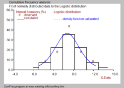
Histogram derived from the adapted cumulative probability distributionHistogram and probability density function, derived from the cumulative probability distribution, for a logistic distribution.
The observed data can be arranged in classes or groups with serial number k. Each group has a lower limit (Lk) and an upper limit (Uk). When the class (k) contains mk data and the total number of data is N, then the relative class or group frequency is found from:
Fg(Lk < X ≤ Uk) = mk / N
or briefly:
Fgk = m/N
or in percentage:
Fg(%) = 100m/N
The presentation of all class frequencies gives a frequency distribution, or histogram. Histograms, even when made from the same record, are different for different class limits.
The histogram can also be derived from the fitted cumulative probability distribution:
Pgk = Pc(Uk) − Pc(Lk)
There may be a difference between Fgk and Pgk due to the deviations of the observed data from the fitted distribution (see blue figure).
Often it is desired to combine the histogram with a probability density function as depicted in the black and white picture.
1 2 Benson, M.A. 1960. Characteristics of frequency curves based on a theoretical 1000-year record. In: T.Dalrymple (ed.), Flood frequency analysis. U.S. Geological Survey Water Supply paper 1543-A, pp. 51–71
1 2 3 4 Frequency and Regression Analysis. Chapter 6 in: H.P. Ritzema (ed., 1994), Drainage Principles and Applications, Publ. 16, pp. 175–224, International Institute for Land Reclamation and Improvement (ILRI), Wageningen, The Netherlands. ISBN90-70754-33-9 . Free download from the webpage under nr. 12, or directly as PDF:
↑ Ghosh, B.K (1979). "A comparison of some approximate confidence intervals for the binomial parameter". Journal of the American Statistical Association. 74 (368): 894–900. doi:10.1080/01621459.1979.10481051.
↑ Blyth, C.R.; H.A. Still (1983). "Binomial confidence intervals". Journal of the American Statistical Association. 78 (381): 108–116. doi:10.1080/01621459.1983.10477938.
↑ Agresti, A.; B. Caffo (2000). "Simple and effective confidence intervals for pro- portions and differences of proportions result from adding two successes and two failures". The American Statistician. 54 (4): 280–288. doi:10.1080/00031305.2000.10474560. S2CID18880883.
↑ Wilson, E.B. (1927). "Probable inference, the law of succession, and statistical inference". Journal of the American Statistical Association. 22 (158): 209–212. doi:10.1080/01621459.1927.10502953.
↑ Hogg, R.V. (2001). Probability and statistical inference (6thed.). Prentice Hall, NJ: Upper Saddle River.
This page is based on this Wikipedia article Text is available under the CC BY-SA 4.0 license; additional terms may apply. Images, videos and audio are available under their respective licenses.