
In probability theory and statistics, a normal distribution or Gaussian distribution is a type of continuous probability distribution for a real-valued random variable. The general form of its probability density function is The parameter is the mean or expectation of the distribution, while the parameter is the variance. The standard deviation of the distribution is (sigma). A random variable with a Gaussian distribution is said to be normally distributed, and is called a normal deviate.

Superparamagnetism is a form of magnetism which appears in small ferromagnetic or ferrimagnetic nanoparticles. In sufficiently small nanoparticles, magnetization can randomly flip direction under the influence of temperature. The typical time between two flips is called the Néel relaxation time. In the absence of an external magnetic field, when the time used to measure the magnetization of the nanoparticles is much longer than the Néel relaxation time, their magnetization appears to be on average zero; they are said to be in the superparamagnetic state. In this state, an external magnetic field is able to magnetize the nanoparticles, similarly to a paramagnet. However, their magnetic susceptibility is much larger than that of paramagnets.

The Allan variance (AVAR), also known as two-sample variance, is a measure of frequency stability in clocks, oscillators and amplifiers. It is named after David W. Allan and expressed mathematically as . The Allan deviation (ADEV), also known as sigma-tau, is the square root of the Allan variance, .

In probability theory, a log-normal (or lognormal) distribution is a continuous probability distribution of a random variable whose logarithm is normally distributed. Thus, if the random variable X is log-normally distributed, then Y = ln(X) has a normal distribution. Equivalently, if Y has a normal distribution, then the exponential function of Y, X = exp(Y), has a log-normal distribution. A random variable which is log-normally distributed takes only positive real values. It is a convenient and useful model for measurements in exact and engineering sciences, as well as medicine, economics and other topics (e.g., energies, concentrations, lengths, prices of financial instruments, and other metrics).
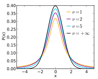
In probability theory and statistics, Student's t distribution is a continuous probability distribution that generalizes the standard normal distribution. Like the latter, it is symmetric around zero and bell-shaped.
In probability theory, Chebyshev's inequality provides an upper bound on the probability of deviation of a random variable from its mean. More specifically, the probability that a random variable deviates from its mean by more than is at most , where is any positive constant and is the standard deviation.

In probability theory and statistics, the Gumbel distribution is used to model the distribution of the maximum of a number of samples of various distributions.
In mathematics, the moments of a function are certain quantitative measures related to the shape of the function's graph. If the function represents mass density, then the zeroth moment is the total mass, the first moment is the center of mass, and the second moment is the moment of inertia. If the function is a probability distribution, then the first moment is the expected value, the second central moment is the variance, the third standardized moment is the skewness, and the fourth standardized moment is the kurtosis.
In statistical inference, specifically predictive inference, a prediction interval is an estimate of an interval in which a future observation will fall, with a certain probability, given what has already been observed. Prediction intervals are often used in regression analysis.

In signal processing, cross-correlation is a measure of similarity of two series as a function of the displacement of one relative to the other. This is also known as a sliding dot product or sliding inner-product. It is commonly used for searching a long signal for a shorter, known feature. It has applications in pattern recognition, single particle analysis, electron tomography, averaging, cryptanalysis, and neurophysiology. The cross-correlation is similar in nature to the convolution of two functions. In an autocorrelation, which is the cross-correlation of a signal with itself, there will always be a peak at a lag of zero, and its size will be the signal energy.
In statistics, a generalized linear model (GLM) is a flexible generalization of ordinary linear regression. The GLM generalizes linear regression by allowing the linear model to be related to the response variable via a link function and by allowing the magnitude of the variance of each measurement to be a function of its predicted value.
Compartmental models are a very general modelling technique. They are often applied to the mathematical modelling of infectious diseases. The population is assigned to compartments with labels – for example, S, I, or R,. People may progress between compartments. The order of the labels usually shows the flow patterns between the compartments; for example SEIS means susceptible, exposed, infectious, then susceptible again.
Variational Bayesian methods are a family of techniques for approximating intractable integrals arising in Bayesian inference and machine learning. They are typically used in complex statistical models consisting of observed variables as well as unknown parameters and latent variables, with various sorts of relationships among the three types of random variables, as might be described by a graphical model. As typical in Bayesian inference, the parameters and latent variables are grouped together as "unobserved variables". Variational Bayesian methods are primarily used for two purposes:
- To provide an analytical approximation to the posterior probability of the unobserved variables, in order to do statistical inference over these variables.
- To derive a lower bound for the marginal likelihood of the observed data. This is typically used for performing model selection, the general idea being that a higher marginal likelihood for a given model indicates a better fit of the data by that model and hence a greater probability that the model in question was the one that generated the data.
In probability and statistics, a circular distribution or polar distribution is a probability distribution of a random variable whose values are angles, usually taken to be in the range [0, 2π). A circular distribution is often a continuous probability distribution, and hence has a probability density, but such distributions can also be discrete, in which case they are called circular lattice distributions. Circular distributions can be used even when the variables concerned are not explicitly angles: the main consideration is that there is not usually any real distinction between events occurring at the opposite ends of the range, and the division of the range could notionally be made at any point.
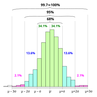
In statistics, the 68–95–99.7 rule, also known as the empirical rule, and sometimes abbreviated 3sr, is a shorthand used to remember the percentage of values that lie within an interval estimate in a normal distribution: approximately 68%, 95%, and 99.7% of the values lie within one, two, and three standard deviations of the mean, respectively.
In actuarial science and applied probability, ruin theory uses mathematical models to describe an insurer's vulnerability to insolvency/ruin. In such models key quantities of interest are the probability of ruin, distribution of surplus immediately prior to ruin and deficit at time of ruin.
In probability theory and statistics, the index of dispersion, dispersion index, coefficient of dispersion, relative variance, or variance-to-mean ratio (VMR), like the coefficient of variation, is a normalized measure of the dispersion of a probability distribution: it is a measure used to quantify whether a set of observed occurrences are clustered or dispersed compared to a standard statistical model.

In probability theory and statistics, the Poisson distribution is a discrete probability distribution that expresses the probability of a given number of events occurring in a fixed interval of time if these events occur with a known constant mean rate and independently of the time since the last event. It can also be used for the number of events in other types of intervals than time, and in dimension greater than 1.
In the theory of renewal processes, a part of the mathematical theory of probability, the residual time or the forward recurrence time is the time between any given time and the next epoch of the renewal process under consideration. In the context of random walks, it is also known as overshoot. Another way to phrase residual time is "how much more time is there to wait?".
An intensity-duration-frequency curve is a mathematical function that relates the intensity of an event with its duration and frequency of occurrence. Frequency is the inverse of the probability of occurrence. These curves are commonly used in hydrology for flood forecasting and civil engineering for urban drainage design. However, the IDF curves are also analysed in hydrometeorology because of the interest in the time concentration or time-structure of the rainfall, but it is also possible to define IDF curves for drought events. Additionally, applications of IDF curves to risk-based design are emerging outside of hydrometeorology, for example some authors developed IDF curves for food supply chain inflow shocks to US cities.


