In computer science, a selection algorithm is an algorithm for finding the th smallest value in a collection of ordered values, such as numbers. The value that it finds is called the th order statistic. Selection includes as special cases the problems of finding the minimum, median, and maximum element in the collection. Selection algorithms include quickselect, and the median of medians algorithm. When applied to a collection of values, these algorithms take linear time, as expressed using big O notation. For data that is already structured, faster algorithms may be possible; as an extreme case, selection in an already-sorted array takes time .

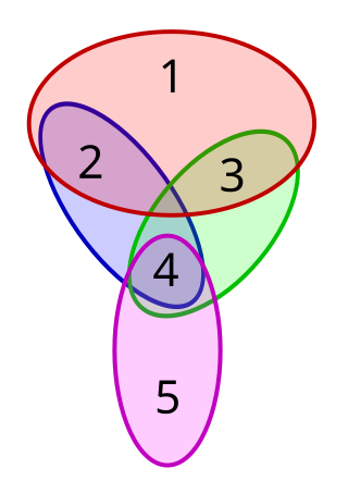
The set cover problem is a classical question in combinatorics, computer science, operations research, and complexity theory.

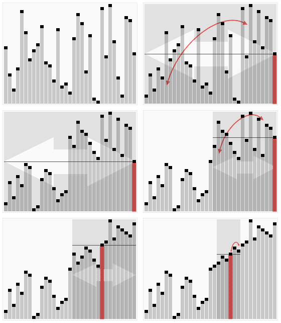
In computer science, quickselect is a selection algorithm to find the kth smallest element in an unordered list, also known as the kth order statistic. Like the related quicksort sorting algorithm, it was developed by Tony Hoare, and thus is also known as Hoare's selection algorithm. Like quicksort, it is efficient in practice and has good average-case performance, but has poor worst-case performance. Quickselect and its variants are the selection algorithms most often used in efficient real-world implementations.

Quicksort is an efficient, general-purpose sorting algorithm. Quicksort was developed by British computer scientist Tony Hoare in 1959 and published in 1961. It is still a commonly used algorithm for sorting. Overall, it is slightly faster than merge sort and heapsort for randomized data, particularly on larger distributions.
In numerical analysis and linear algebra, lower–upper (LU) decomposition or factorization factors a matrix as the product of a lower triangular matrix and an upper triangular matrix. The product sometimes includes a permutation matrix as well. LU decomposition can be viewed as the matrix form of Gaussian elimination. Computers usually solve square systems of linear equations using LU decomposition, and it is also a key step when inverting a matrix or computing the determinant of a matrix. The LU decomposition was introduced by the Polish astronomer Tadeusz Banachiewicz in 1938. To quote: "It appears that Gauss and Doolittle applied the method [of elimination] only to symmetric equations. More recent authors, for example, Aitken, Banachiewicz, Dwyer, and Crout … have emphasized the use of the method, or variations of it, in connection with non-symmetric problems … Banachiewicz … saw the point … that the basic problem is really one of matrix factorization, or “decomposition” as he called it." It is also sometimes referred to as LR decomposition.
The sample mean or empirical mean, and the sample covariance or empirical covariance are statistics computed from a sample of data on one or more random variables.

In geometry, the geometric median of a discrete set of sample points in a Euclidean space is the point minimizing the sum of distances to the sample points. This generalizes the median, which has the property of minimizing the sum of distances for one-dimensional data, and provides a central tendency in higher dimensions. It is also known as the spatial median, Euclidean minisum point, Torricelli point, or 1-median.

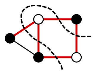
In a graph, a maximum cut is a cut whose size is at least the size of any other cut. That is, it is a partition of the graph's vertices into two complementary sets S and T, such that the number of edges between S and T is as large as possible. Finding such a cut is known as the max-cut problem.
Clustering is the problem of partitioning data points into groups based on their similarity. Correlation clustering provides a method for clustering a set of objects into the optimum number of clusters without specifying that number in advance.
In mathematics, the Robinson–Schensted–Knuth correspondence, also referred to as the RSK correspondence or RSK algorithm, is a combinatorial bijection between matrices A with non-negative integer entries and pairs (P,Q) of semistandard Young tableaux of equal shape, whose size equals the sum of the entries of A. More precisely the weight of P is given by the column sums of A, and the weight of Q by its row sums. It is a generalization of the Robinson–Schensted correspondence, in the sense that taking A to be a permutation matrix, the pair (P,Q) will be the pair of standard tableaux associated to the permutation under the Robinson–Schensted correspondence.
In combinatorial optimization, the matroid intersection problem is to find a largest common independent set in two matroids over the same ground set. If the elements of the matroid are assigned real weights, the weighted matroid intersection problem is to find a common independent set with the maximum possible weight. These problems generalize many problems in combinatorial optimization including finding maximum matchings and maximum weight matchings in bipartite graphs and finding arborescences in directed graphs.
The Davies–Bouldin index (DBI), introduced by David L. Davies and Donald W. Bouldin in 1979, is a metric for evaluating clustering algorithms. This is an internal evaluation scheme, where the validation of how well the clustering has been done is made using quantities and features inherent to the dataset. This has a drawback that a good value reported by this method does not imply the best information retrieval.
In computer science, the range query problem consists of efficiently answering several queries regarding a given interval of elements within an array. For example, a common task, known as range minimum query, is finding the smallest value inside a given range within a list of numbers.

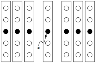
In computer science, the median of medians is an approximate median selection algorithm, frequently used to supply a good pivot for an exact selection algorithm, most commonly quickselect, that selects the kth smallest element of an initially unsorted array. Median of medians finds an approximate median in linear time. Using this approximate median as an improved pivot, the worst-case complexity of quickselect reduces from quadratic to linear, which is also the asymptotically optimal worst-case complexity of any selection algorithm. In other words, the median of medians is an approximate median-selection algorithm that helps building an asymptotically optimal, exact general selection algorithm, by producing good pivot elements.
In computer science, an optimal binary search tree (Optimal BST), sometimes called a weight-balanced binary tree, is a binary search tree which provides the smallest possible search time (or expected search time) for a given sequence of accesses (or access probabilities). Optimal BSTs are generally divided into two types: static and dynamic.
The cache-oblivious distribution sort is a comparison-based sorting algorithm. It is similar to quicksort, but it is a cache-oblivious algorithm, designed for a setting where the number of elements to sort is too large to fit in a cache where operations are done. In the external memory model, the number of memory transfers it needs to perform a sort of items on a machine with cache of size and cache lines of length is , under the tall cache assumption that . This number of memory transfers has been shown to be asymptotically optimal for comparison sorts. This distribution sort also achieves the asymptotically optimal runtime complexity of .

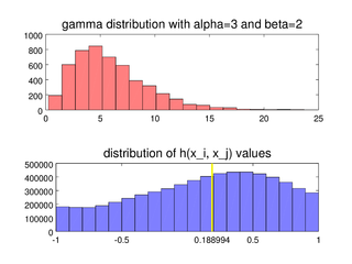
In statistics, the medcouple is a robust statistic that measures the skewness of a univariate distribution. It is defined as a scaled median difference between the left and right half of a distribution. Its robustness makes it suitable for identifying outliers in adjusted boxplots. Ordinary box plots do not fare well with skew distributions, since they label the longer unsymmetrical tails as outliers. Using the medcouple, the whiskers of a boxplot can be adjusted for skew distributions and thus have a more accurate identification of outliers for non-symmetrical distributions.
In the fair cake-cutting problem, the partners often have different entitlements. For example, the resource may belong to two shareholders such that Alice holds 8/13 and George holds 5/13. This leads to the criterion of weighted proportionality (WPR): there are several weights that sum up to 1, and every partner should receive at least a fraction of the resource by their own valuation.

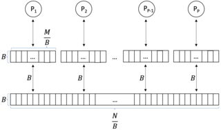
In computer science, a parallel external memory (PEM) model is a cache-aware, external-memory abstract machine. It is the parallel-computing analogy to the single-processor external memory (EM) model. In a similar way, it is the cache-aware analogy to the parallel random-access machine (PRAM). The PEM model consists of a number of processors, together with their respective private caches and a shared main memory.
In computer science, multiway number partitioning is the problem of partitioning a multiset of numbers into a fixed number of subsets, such that the sums of the subsets are as similar as possible. It was first presented by Ronald Graham in 1969 in the context of the identical-machines scheduling problem. The problem is parametrized by a positive integer k, and called k-way number partitioning. The input to the problem is a multiset S of numbers, whose sum is k*T.


