Least absolute deviations

Last updated November 24, 2023

Least absolute deviations (LAD), also known as least absolute errors (LAE), least absolute residuals (LAR), or least absolute values (LAV), is a statistical optimality criterion and a statistical optimization technique based on minimizing the sum of absolute deviations (also sum of absolute residuals or sum of absolute errors) or the L₁ norm of such values. It is analogous to the least squares technique, except that it is based on absolute values instead of squared values. It attempts to find a function which closely approximates a set of data by minimizing residuals between points generated by the function and corresponding data points. The LAD estimate also arises as the maximum likelihood estimate if the errors have a Laplace distribution. It was introduced in 1757 by Roger Joseph Boscovich.^[1]

Formulation

Suppose that the data set consists of the points (x_i, y_i) with i = 1, 2, ..., n. We want to find a function f such that $f(x_{i})\approx y_{i}.$

To attain this goal, we suppose that the function f is of a particular form containing some parameters that need to be determined. For instance, the simplest form would be linear: f(x) = bx + c, where b and c are parameters whose values are not known but which we would like to estimate. Less simply, suppose that f(x) is quadratic, meaning that f(x) = ax² + bx + c, where a, b and c are not yet known. (More generally, there could be not just one explanator x, but rather multiple explanators, all appearing as arguments of the function f.)

We now seek estimated values of the unknown parameters that minimize the sum of the absolute values of the residuals:

S=\sum _{i=1}^{n}|y_{i}-f(x_{i})|.

Solution

Though the idea of least absolute deviations regression is just as straightforward as that of least squares regression, the least absolute deviations line is not as simple to compute efficiently. Unlike least squares regression, least absolute deviations regression does not have an analytical solving method. Therefore, an iterative approach is required. The following is an enumeration of some least absolute deviations solving methods.

Simplex-based methods (such as the Barrodale-Roberts algorithm^[2])
- Because the problem is a linear program, any of the many linear programming techniques (including the simplex method as well as others) can be applied.
Iteratively re-weighted least squares ^[3]
Wesolowsky's direct descent method^[4]
Li-Arce's maximum likelihood approach^[5]
Recursive reduction of dimensionality approach^[6]
Check all combinations of point-to-point lines for minimum sum of errors

Simplex-based methods are the “preferred” way to solve the least absolute deviations problem.^[7] A Simplex method is a method for solving a problem in linear programming. The most popular algorithm is the Barrodale-Roberts modified Simplex algorithm. The algorithms for IRLS, Wesolowsky's Method, and Li's Method can be found in Appendix A of ^[7] among other methods. Checking all combinations of lines traversing any two (x,y) data points is another method of finding the least absolute deviations line. Since it is known that at least one least absolute deviations line traverses at least two data points, this method will find a line by comparing the SAE (Smallest Absolute Error over data points) of each line, and choosing the line with the smallest SAE. In addition, if multiple lines have the same, smallest SAE, then the lines outline the region of multiple solutions. Though simple, this final method is inefficient for large sets of data.

Solution using linear programming

The problem can be solved using any linear programming technique on the following problem specification. We wish to

{\text{Minimize}}\sum _{i=1}^{n}|y_{i}-a_{0}-a_{1}x_{i1}-a_{2}x_{i2}-\cdots -a_{k}x_{ik}|

with respect to the choice of the values of the parameters $a_{0},\ldots ,a_{k}$ , where y_i is the value of the i^th observation of the dependent variable, and x_ij is the value of the i^th observation of the j^th independent variable (j = 1,...,k). We rewrite this problem in terms of artificial variables u_i as

{\text{Minimize}}\sum _{i=1}^{n}u_{i}

with respect to

a_{0},\ldots ,a_{k}

and

u_{1},\ldots ,u_{n}

subject to

u_{i}\geq y_{i}-a_{0}-a_{1}x_{i1}-a_{2}x_{i2}-\cdots -a_{k}x_{ik}\,\ \,\ \,\ \,\ \,\ {\text{for }}i=1,\ldots ,n

u_{i}\geq -[y_{i}-a_{0}-a_{1}x_{i1}-a_{2}x_{i2}-\cdots -a_{k}x_{ik}]\,\ \,\ {\text{ for }}i=1,\ldots ,n.

These constraints have the effect of forcing each $u_{i}$ to equal $|y_{i}-a_{0}-a_{1}x_{i1}-a_{2}x_{i2}-\cdots -a_{k}x_{ik}|$ upon being minimized, so the objective function is equivalent to the original objective function. Since this version of the problem statement does not contain the absolute value operator, it is in a format that can be solved with any linear programming package.

Properties

There exist other unique properties of the least absolute deviations line. In the case of a set of (x,y) data, the least absolute deviations line will always pass through at least two of the data points, unless there are multiple solutions. If multiple solutions exist, then the region of valid least absolute deviations solutions will be bounded by at least two lines, each of which passes through at least two data points. More generally, if there are k regressors (including the constant), then at least one optimal regression surface will pass through k of the data points.^[8]^: p.936

This "latching" of the line to the data points can help to understand the "instability" property: if the line always latches to at least two points, then the line will jump between different sets of points as the data points are altered. The "latching" also helps to understand the "robustness" property: if there exists an outlier, and a least absolute deviations line must latch onto two data points, the outlier will most likely not be one of those two points because that will not minimize the sum of absolute deviations in most cases.

One known case in which multiple solutions exist is a set of points symmetric about a horizontal line, as shown in Figure A below.

Figure A: A set of data points with reflection symmetry and multiple least absolute deviations solutions. The "solution area" is shown in green. The vertical blue lines represent the absolute errors from the pink line to each data point. The pink line is one of infinitely many solutions within the green area. Least absolute deviations regression method diagram.gif — Figure A: A set of data points with reflection symmetry and multiple least absolute deviations solutions. The “solution area” is shown in green. The vertical blue lines represent the absolute errors from the pink line to each data point. The pink line is one of infinitely many solutions within the green area.

To understand why there are multiple solutions in the case shown in Figure A, consider the pink line in the green region. Its sum of absolute errors is some value S. If one were to tilt the line upward slightly, while still keeping it within the green region, the sum of errors would still be S. It would not change because the distance from each point to the line grows on one side of the line, while the distance to each point on the opposite side of the line diminishes by exactly the same amount. Thus the sum of absolute errors remains the same. Also, since one can tilt the line in infinitely small increments, this also shows that if there is more than one solution, there are infinitely many solutions.

Advantages and disadvantages

The following is a table contrasting some properties of the method of least absolute deviations with those of the method of least squares (for non-singular problems).^[9]^[10]

Ordinary least squares regression	Least absolute deviations regression
Not very robust	Robust
Stable solution	Unstable solution
One solution*	Possibly multiple solutions

*Provided that the number of data points is greater than or equal to the number of features.

The method of least absolute deviations finds applications in many areas, due to its robustness compared to the least squares method. Least absolute deviations is robust in that it is resistant to outliers in the data. LAD gives equal emphasis to all observations, in contrast to ordinary least squares (OLS) which, by squaring the residuals, gives more weight to large residuals, that is, outliers in which predicted values are far from actual observations. This may be helpful in studies where outliers do not need to be given greater weight than other observations. If it is important to give greater weight to outliers, the method of least squares is a better choice.

Variations, extensions, specializations

If in the sum of the absolute values of the residuals one generalises the absolute value function to a tilted absolute value function, which on the left half-line has slope $\tau -1$ and on the right half-line has slope $\tau$ , where $0<\tau <1$ , one obtains quantile regression. The case of $\tau =1/2$ gives the standard regression by least absolute deviations and is also known as median regression .

The least absolute deviation problem may be extended to include multiple explanators, constraints and regularization, e.g., a linear model with linear constraints:^[11]

minimize

S(\mathbf {\beta } ,b)=\sum _{i}|\mathbf {x} '_{i}\mathbf {\beta } +b-y_{i}|

subject to, e.g.,

\mathbf {x} '_{1}\mathbf {\beta } +b-y_{1}\leq k

where $\mathbf {\beta }$ is a column vector of coefficients to be estimated, b is an intercept to be estimated, x_i is a column vector of the i^th observations on the various explanators, y_i is the i^th observation on the dependent variable, and k is a known constant.

Regularization with LASSO (least absolute shrinkage and selection operator) may also be combined with LAD.^[12]

Related Research Articles

The method of least squares is a standard approach in regression analysis to approximate the solution of overdetermined systems by minimizing the sum of the squares of the residuals made in the results of each individual equation.

In statistics, the Gauss–Markov theorem states that the ordinary least squares (OLS) estimator has the lowest sampling variance within the class of linear unbiased estimators, if the errors in the linear regression model are uncorrelated, have equal variances and expectation value of zero. The errors do not need to be normal, nor do they need to be independent and identically distributed. The requirement that the estimator be unbiased cannot be dropped, since biased estimators exist with lower variance. See, for example, the James–Stein estimator, ridge regression, or simply any degenerate estimator.

In statistics and optimization, errors and residuals are two closely related and easily confused measures of the deviation of an observed value of an element of a statistical sample from its "true value". The error of an observation is the deviation of the observed value from the true value of a quantity of interest. The residual is the difference between the observed value and the estimated value of the quantity of interest. The distinction is most important in regression analysis, where the concepts are sometimes called the regression errors and regression residuals and where they lead to the concept of studentized residuals. In econometrics, "errors" are also called disturbances.

In statistical modeling, regression analysis is a set of statistical processes for estimating the relationships between a dependent variable and one or more independent variables. The most common form of regression analysis is linear regression, in which one finds the line that most closely fits the data according to a specific mathematical criterion. For example, the method of ordinary least squares computes the unique line that minimizes the sum of squared differences between the true data and that line. For specific mathematical reasons, this allows the researcher to estimate the conditional expectation of the dependent variable when the independent variables take on a given set of values. Less common forms of regression use slightly different procedures to estimate alternative location parameters or estimate the conditional expectation across a broader collection of non-linear models.

In mathematics and computing, the Levenberg–Marquardt algorithm, also known as the damped least-squares (DLS) method, is used to solve non-linear least squares problems. These minimization problems arise especially in least squares curve fitting. The LMA interpolates between the Gauss–Newton algorithm (GNA) and the method of gradient descent. The LMA is more robust than the GNA, which means that in many cases it finds a solution even if it starts very far off the final minimum. For well-behaved functions and reasonable starting parameters, the LMA tends to be slower than the GNA. LMA can also be viewed as Gauss–Newton using a trust region approach.

Ridge regression is a method of estimating the coefficients of multiple-regression models in scenarios where the independent variables are highly correlated. It has been used in many fields including econometrics, chemistry, and engineering. Also known as Tikhonov regularization, named for Andrey Tikhonov, it is a method of regularization of ill-posed problems. It is particularly useful to mitigate the problem of multicollinearity in linear regression, which commonly occurs in models with large numbers of parameters. In general, the method provides improved efficiency in parameter estimation problems in exchange for a tolerable amount of bias.

In applied statistics, total least squares is a type of errors-in-variables regression, a least squares data modeling technique in which observational errors on both dependent and independent variables are taken into account. It is a generalization of Deming regression and also of orthogonal regression, and can be applied to both linear and non-linear models.

In statistics, nonlinear regression is a form of regression analysis in which observational data are modeled by a function which is a nonlinear combination of the model parameters and depends on one or more independent variables. The data are fitted by a method of successive approximations.

The Gauss–Newton algorithm is used to solve non-linear least squares problems, which is equivalent to minimizing a sum of squared function values. It is an extension of Newton's method for finding a minimum of a non-linear function. Since a sum of squares must be nonnegative, the algorithm can be viewed as using Newton's method to iteratively approximate zeroes of the components of the sum, and thus minimizing the sum. In this sense, the algorithm is also an effective method for solving overdetermined systems of equations. It has the advantage that second derivatives, which can be challenging to compute, are not required.

In statistics, ordinary least squares (OLS) is a type of linear least squares method for choosing the unknown parameters in a linear regression model by the principle of least squares: minimizing the sum of the squares of the differences between the observed dependent variable in the input dataset and the output of the (linear) function of the independent variable.

Weighted least squares (WLS), also known as weighted linear regression, is a generalization of ordinary least squares and linear regression in which knowledge of the unequal variance of observations (heteroscedasticity) is incorporated into the regression. WLS is also a specialization of generalized least squares, when all the off-diagonal entries of the covariance matrix of the errors, are null.

In statistics, the residual sum of squares (RSS), also known as the sum of squared residuals (SSR) or the sum of squared estimate of errors (SSE), is the sum of the squares of residuals. It is a measure of the discrepancy between the data and an estimation model, such as a linear regression. A small RSS indicates a tight fit of the model to the data. It is used as an optimality criterion in parameter selection and model selection.

In statistics, simple linear regression is a linear regression model with a single explanatory variable. That is, it concerns two-dimensional sample points with one independent variable and one dependent variable and finds a linear function that, as accurately as possible, predicts the dependent variable values as a function of the independent variable. The adjective simple refers to the fact that the outcome variable is related to a single predictor.

In robust statistics, robust regression seeks to overcome some limitations of traditional regression analysis. A regression analysis models the relationship between one or more independent variables and a dependent variable. Standard types of regression, such as ordinary least squares, have favourable properties if their underlying assumptions are true, but can give misleading results otherwise. Robust regression methods are designed to limit the effect that violations of assumptions by the underlying data-generating process have on regression estimates.

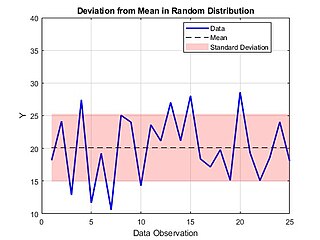
The method of iteratively reweighted least squares (IRLS) is used to solve certain optimization problems with objective functions of the form of a p-norm:

<span class="mw-page-title-main">Quantile regression</span> Statistics concept

Quantile regression is a type of regression analysis used in statistics and econometrics. Whereas the method of least squares estimates the conditional mean of the response variable across values of the predictor variables, quantile regression estimates the conditional median of the response variable. Quantile regression is an extension of linear regression used when the conditions of linear regression are not met.

Non-linear least squares is the form of least squares analysis used to fit a set of m observations with a model that is non-linear in n unknown parameters (m ≥ n). It is used in some forms of nonlinear regression. The basis of the method is to approximate the model by a linear one and to refine the parameters by successive iterations. There are many similarities to linear least squares, but also some significant differences. In economic theory, the non-linear least squares method is applied in (i) the probit regression, (ii) threshold regression, (iii) smooth regression, (iv) logistic link regression, (v) Box–Cox transformed regressors ( $).$

Least trimmed squares (LTS), or least trimmed sum of squares, is a robust statistical method that fits a function to a set of data whilst not being unduly affected by the presence of outliers. It is one of a number of methods for robust regression.

Linear least squares (LLS) is the least squares approximation of linear functions to data. It is a set of formulations for solving statistical problems involved in linear regression, including variants for ordinary (unweighted), weighted, and generalized (correlated) residuals. Numerical methods for linear least squares include inverting the matrix of the normal equations and orthogonal decomposition methods.

In statistics, linear regression is a linear approach for modelling the relationship between a scalar response and one or more explanatory variables. The case of one explanatory variable is called simple linear regression; for more than one, the process is called multiple linear regression. This term is distinct from multivariate linear regression, where multiple correlated dependent variables are predicted, rather than a single scalar variable.

References

↑ "Least Absolute Deviation Regression". The Concise Encyclopedia of Statistics . Springer. 2008. pp. 299–302. doi:10.1007/978-0-387-32833-1_225. ISBN 9780387328331.
↑ Barrodale, I.; Roberts, F. D. K. (1973). "An improved algorithm for discrete L₁ linear approximation". SIAM Journal on Numerical Analysis . 10 (5): 839–848. Bibcode:1973SJNA...10..839B. doi:10.1137/0710069. hdl: 1828/11491 . JSTOR 2156318.
↑ Schlossmacher, E. J. (December 1973). "An Iterative Technique for Absolute Deviations Curve Fitting". Journal of the American Statistical Association . 68 (344): 857–859. doi:10.2307/2284512. JSTOR 2284512.
↑ Wesolowsky, G. O. (1981). "A new descent algorithm for the least absolute value regression problem". Communications in Statistics – Simulation and Computation. B10 (5): 479–491. doi:10.1080/03610918108812224.
↑ Li, Yinbo; Arce, Gonzalo R. (2004). "A Maximum Likelihood Approach to Least Absolute Deviation Regression". EURASIP Journal on Applied Signal Processing . 2004 (12): 1762–1769. Bibcode:2004EJASP2004...61L. doi: 10.1155/S1110865704401139 .
↑ Kržić, Ana Sović; Seršić, Damir (2018). "L1 minimization using recursive reduction of dimensionality". Signal Processing. 151: 119–129. doi:10.1016/j.sigpro.2018.05.002.
1 2 William A. Pfeil, Statistical Teaching Aids , Bachelor of Science thesis, Worcester Polytechnic Institute, 2006
↑ Branham, R. L., Jr., "Alternatives to least squares", Astronomical Journal 87, June 1982, 928–937. at SAO/NASA Astrophysics Data System (ADS)
↑ For a set of applets that demonstrate these differences, see the following site: http://www.math.wpi.edu/Course_Materials/SAS/lablets/7.3/73_choices.html
↑ For a discussion of LAD versus OLS, see these academic papers and reports: http://www.econ.uiuc.edu/~roger/research/rq/QRJEP.pdf and https://www.leeds.ac.uk/educol/documents/00003759.htm
↑ Shi, Mingren; Mark A., Lukas (March 2002). "An L₁ estimation algorithm with degeneracy and linear constraints". Computational Statistics & Data Analysis . 39 (1): 35–55. doi:10.1016/S0167-9473(01)00049-4.
↑ Wang, Li; Gordon, Michael D.; Zhu, Ji (December 2006). "Regularized Least Absolute Deviations Regression and an Efficient Algorithm for Parameter Tuning". Proceedings of the Sixth International Conference on Data Mining. pp. 690–700. doi:10.1109/ICDM.2006.134.