Linear regression

For other uses, see Linear regression (disambiguation).

In statistics, linear regression is a model that estimates the linear relationship between a scalar response (dependent variable) and one or more explanatory variables (regressor or independent variable). A model with exactly one explanatory variable is a simple linear regression ; a model with two or more explanatory variables is a multiple linear regression. ^[1] This term is distinct from multivariate linear regression, which predicts multiple correlated dependent variables rather than a single dependent variable. ^[2]

In linear regression, the relationships are modeled using linear predictor functions whose unknown model parameters are estimated from the data. Most commonly, the conditional mean of the response given the values of the explanatory variables (or predictors) is assumed to be an affine function of those values; less commonly, the conditional median or some other quantile is used. Like all forms of regression analysis, linear regression focuses on the conditional probability distribution of the response given the values of the predictors, rather than on the joint probability distribution of all of these variables, which is the domain of multivariate analysis.

Linear regression is also a type of machine learning algorithm, more specifically a supervised algorithm, that learns from the labelled datasets and maps the data points to the most optimized linear functions that can be used for prediction on new datasets. ^[3]

Linear regression was the first type of regression analysis to be studied rigorously, and to be used extensively in practical applications. ^[4] This is because models which depend linearly on their unknown parameters are easier to fit than models which are non-linearly related to their parameters and because the statistical properties of the resulting estimators are easier to determine.

Linear regression has many practical uses. Most applications fall into one of the following two broad categories:

• If the goal is error i.e. variance reduction in prediction or forecasting, linear regression can be used to fit a predictive model to an observed data set of values of the response and explanatory variables. After developing such a model, if additional values of the explanatory variables are collected without an accompanying response value, the fitted model can be used to make a prediction of the response.
• If the goal is to explain variation in the response variable that can be attributed to variation in the explanatory variables, linear regression analysis can be applied to quantify the strength of the relationship between the response and the explanatory variables, and in particular to determine whether some explanatory variables may have no linear relationship with the response at all, or to identify which subsets of explanatory variables may contain redundant information about the response.

Linear regression models are often fitted using the least squares approach, but they may also be fitted in other ways, such as by minimizing the "lack of fit" in some other norm (as with least absolute deviations regression), or by minimizing a penalized version of the least squares cost function as in ridge regression (L²-norm penalty) and lasso (L¹-norm penalty). Use of the Mean Squared Error (MSE) as the cost on a dataset that has many large outliers, can result in a model that fits the outliers more than the true data due to the higher importance assigned by MSE to large errors. So, cost functions that are robust to outliers should be used if the dataset has many large outliers. Conversely, the least squares approach can be used to fit models that are not linear models. Thus, although the terms "least squares" and "linear model" are closely linked, they are not synonymous.

Formulation

In linear regression, the observations (red) are assumed to be the result of random deviations (green) from an underlying relationship (blue) between a dependent variable (y) and an independent variable (x).

Given a data set ${\displaystyle \{y_{i},\,x_{i1},\ldots ,x_{ip}\}_{i=1}^{n}}$ of n statistical units, a linear regression model assumes that the relationship between the dependent variable y and the vector of regressors x is linear. This relationship is modeled through a disturbance term or error variableε—an unobserved random variable that adds "noise" to the linear relationship between the dependent variable and regressors. Thus the model takes the form$${\displaystyle y_{i}=\beta _{0}+\beta _{1}x_{i1}+\cdots +\beta _{p}x_{ip}+\varepsilon _{i}=\mathbf {x} _{i}^{\mathsf {T}}{\boldsymbol {\beta }}+\varepsilon _{i},\qquad i=1,\ldots ,n,}$$where ^T denotes the transpose, so that x_i^Tβ is the inner product between vectors x_i and β.

Often these n equations are stacked together and written in matrix notation as

${\displaystyle \mathbf {y} =\mathbf {X} {\boldsymbol {\beta }}+{\boldsymbol {\varepsilon }},\,}$

where

${\displaystyle \mathbf {y} ={\begin{bmatrix}y_{1}\\y_{2}\\\vdots \\y_{n}\end{bmatrix}},\quad }$

${\displaystyle \mathbf {X} ={\begin{bmatrix}\mathbf {x} _{1}^{\mathsf {T}}\\\mathbf {x} _{2}^{\mathsf {T}}\\\vdots \\\mathbf {x} _{n}^{\mathsf {T}}\end{bmatrix}}={\begin{bmatrix}1&x_{11}&\cdots &x_{1p}\\1&x_{21}&\cdots &x_{2p}\\\vdots &\vdots &\ddots &\vdots \\1&x_{n1}&\cdots &x_{np}\end{bmatrix}},}$

${\displaystyle {\boldsymbol {\beta }}={\begin{bmatrix}\beta _{0}\\\beta _{1}\\\beta _{2}\\\vdots \\\beta _{p}\end{bmatrix}},\quad {\boldsymbol {\varepsilon }}={\begin{bmatrix}\varepsilon _{1}\\\varepsilon _{2}\\\vdots \\\varepsilon _{n}\end{bmatrix}}.}$

Notation and terminology

• ${\displaystyle \mathbf {y} }$ is a vector of observed values ${\displaystyle y_{i}\ (i=1,\ldots ,n)}$ of the variable called the regressand, endogenous variable, response variable, target variable, measured variable, criterion variable, or dependent variable . This variable is also sometimes known as the predicted variable, but this should not be confused with predicted values, which are denoted ${\displaystyle {\hat {y}}}$. The decision as to which variable in a data set is modeled as the dependent variable and which are modeled as the independent variables may be based on a presumption that the value of one of the variables is caused by, or directly influenced by the other variables. Alternatively, there may be an operational reason to model one of the variables in terms of the others, in which case there need be no presumption of causality.
• ${\displaystyle \mathbf {X} }$ may be seen as a matrix of row-vectors ${\displaystyle \mathbf {x} _{i\cdot }}$ or of n-dimensional column-vectors ${\displaystyle \mathbf {x} _{\cdot j}}$, which are known as regressors, exogenous variables, explanatory variables, covariates, input variables, predictor variables, or independent variables (not to be confused with the concept of independent random variables). The matrix ${\displaystyle \mathbf {X} }$ is sometimes called the design matrix .
  • Usually a constant is included as one of the regressors. In particular, ${\displaystyle x_{i0}=1}$ for ${\displaystyle i=1,\ldots ,n}$. The corresponding element of β is called the intercept . Many statistical inference procedures for linear models require an intercept to be present, so it is often included even if theoretical considerations suggest that its value should be zero.
  • Sometimes one of the regressors can be a non-linear function of another regressor or of the data values, as in polynomial regression and segmented regression. The model remains linear as long as it is linear in the parameter vector β.
  • The values x_ij may be viewed as either observed values of random variables X_j or as fixed values chosen prior to observing the dependent variable. Both interpretations may be appropriate in different cases, and they generally lead to the same estimation procedures; however different approaches to asymptotic analysis are used in these two situations.
• ${\displaystyle {\boldsymbol {\beta }}}$ is a ${\displaystyle (p+1)}$-dimensional parameter vector, where ${\displaystyle \beta _{0}}$ is the intercept term (if one is included in the model—otherwise ${\displaystyle {\boldsymbol {\beta }}}$ is p-dimensional). Its elements are known as effects or regression coefficients (although the latter term is sometimes reserved for the estimated effects). In simple linear regression, p=1, and the coefficient is known as regression slope. Statistical estimation and inference in linear regression focuses on β. The elements of this parameter vector are interpreted as the partial derivatives of the dependent variable with respect to the various independent variables.
• ${\displaystyle {\boldsymbol {\varepsilon }}}$ is a vector of values ${\displaystyle \varepsilon _{i}}$. This part of the model is called the error term, disturbance term, or sometimes noise (in contrast with the "signal" provided by the rest of the model). This variable captures all other factors which influence the dependent variable y other than the regressors x. The relationship between the error term and the regressors, for example their correlation, is a crucial consideration in formulating a linear regression model, as it will determine the appropriate estimation method.

Fitting a linear model to a given data set usually requires estimating the regression coefficients ${\displaystyle {\boldsymbol {\beta }}}$ such that the error term ${\displaystyle {\boldsymbol {\varepsilon }}=\mathbf {y} -\mathbf {X} {\boldsymbol {\beta }}}$ is minimized. For example, it is common to use the sum of squared errors ${\displaystyle \|{\boldsymbol {\varepsilon }}\|_{2}^{2}}$ as a measure of ${\displaystyle {\boldsymbol {\varepsilon }}}$ for minimization.

Example

Consider a situation where a small ball is being tossed up in the air and then we measure its heights of ascent h_i at various moments in time t_i. Physics tells us that, ignoring the drag, the relationship can be modeled as

${\displaystyle h_{i}=\beta _{1}t_{i}+\beta _{2}t_{i}^{2}+\varepsilon _{i},}$

where β₁ determines the initial velocity of the ball, β₂ is proportional to the standard gravity, and ε_i is due to measurement errors. Linear regression can be used to estimate the values of β₁ and β₂ from the measured data. This model is non-linear in the time variable, but it is linear in the parameters β₁ and β₂; if we take regressors x_i = (x_i1, x_i2)  = (t_i, t_i²), the model takes on the standard form

${\displaystyle h_{i}=\mathbf {x} _{i}^{\mathsf {T}}{\boldsymbol {\beta }}+\varepsilon _{i}.}$

Assumptions

See also: Ordinary least squares § Assumptions

Standard linear regression models with standard estimation techniques make a number of assumptions about the predictor variables, the response variable and their relationship. Numerous extensions have been developed that allow each of these assumptions to be relaxed (i.e. reduced to a weaker form), and in some cases eliminated entirely. Generally these extensions make the estimation procedure more complex and time-consuming, and may also require more data in order to produce an equally precise model.^{[ citation needed ]}

Example of a cubic polynomial regression, which is a type of linear regression. Although polynomial regression fits a curve model to the data, as a statistical estimation problem it is linear, in the sense that the regression function E(y | x) is linear in the unknown parameters that are estimated from the data. For this reason, polynomial regression is considered to be a special case of multiple linear regression.

The following are the major assumptions made by standard linear regression models with standard estimation techniques (e.g. ordinary least squares):

• Weak exogeneity. This essentially means that the predictor variables x can be treated as fixed values, rather than random variables. This means, for example, that the predictor variables are assumed to be error-free—that is, not contaminated with measurement errors. Although this assumption is not realistic in many settings, dropping it leads to significantly more difficult errors-in-variables models.
• Linearity. This means that the mean of the response variable is a linear combination of the parameters (regression coefficients) and the predictor variables. Note that this assumption is much less restrictive than it may at first seem. Because the predictor variables are treated as fixed values (see above), linearity is really only a restriction on the parameters. The predictor variables themselves can be arbitrarily transformed, and in fact multiple copies of the same underlying predictor variable can be added, each one transformed differently. This technique is used, for example, in polynomial regression, which uses linear regression to fit the response variable as an arbitrary polynomial function (up to a given degree) of a predictor variable. With this much flexibility, models such as polynomial regression often have "too much power", in that they tend to overfit the data. As a result, some kind of regularization must typically be used to prevent unreasonable solutions coming out of the estimation process. Common examples are ridge regression and lasso regression. Bayesian linear regression can also be used, which by its nature is more or less immune to the problem of overfitting. (In fact, ridge regression and lasso regression can both be viewed as special cases of Bayesian linear regression, with particular types of prior distributions placed on the regression coefficients.)

• 

  Visualization of heteroscedasticity in a scatter plot against 100 random fitted values using Matlab

  Constant variance (a.k.a. homoscedasticity ). This means that the variance of the errors does not depend on the values of the predictor variables. Thus the variability of the responses for given fixed values of the predictors is the same regardless of how large or small the responses are. This is often not the case, as a variable whose mean is large will typically have a greater variance than one whose mean is small. For example, a person whose income is predicted to be $100,000 may easily have an actual income of $80,000 or $120,000—i.e., a standard deviation of around $20,000—while another person with a predicted income of $10,000 is unlikely to have the same $20,000 standard deviation, since that would imply their actual income could vary anywhere between −$10,000 and $30,000. (In fact, as this shows, in many cases—often the same cases where the assumption of normally distributed errors fails—the variance or standard deviation should be predicted to be proportional to the mean, rather than constant.) The absence of homoscedasticity is called heteroscedasticity. In order to check this assumption, a plot of residuals versus predicted values (or the values of each individual predictor) can be examined for a "fanning effect" (i.e., increasing or decreasing vertical spread as one moves left to right on the plot). A plot of the absolute or squared residuals versus the predicted values (or each predictor) can also be examined for a trend or curvature. Formal tests can also be used; see Heteroscedasticity. The presence of heteroscedasticity will result in an overall "average" estimate of variance being used instead of one that takes into account the true variance structure. This leads to less precise (but in the case of ordinary least squares, not biased) parameter estimates and biased standard errors, resulting in misleading tests and interval estimates. The mean squared error for the model will also be wrong. Various estimation techniques including weighted least squares and the use of heteroscedasticity-consistent standard errors can handle heteroscedasticity in a quite general way. Bayesian linear regression techniques can also be used when the variance is assumed to be a function of the mean. It is also possible in some cases to fix the problem by applying a transformation to the response variable (e.g., fitting the logarithm of the response variable using a linear regression model, which implies that the response variable itself has a log-normal distribution rather than a normal distribution).

To check for violations of the assumptions of linearity, constant variance, and independence of errors within a linear regression model, the residuals are typically plotted against the predicted values (or each of the individual predictors). An apparently random scatter of points about the horizontal midline at 0 is ideal, but cannot rule out certain kinds of violations such as autocorrelation in the errors or their correlation with one or more covariates.

• Independence of errors. This assumes that the errors of the response variables are uncorrelated with each other. (Actual statistical independence is a stronger condition than mere lack of correlation and is often not needed, although it can be exploited if it is known to hold.) Some methods such as generalized least squares are capable of handling correlated errors, although they typically require significantly more data unless some sort of regularization is used to bias the model towards assuming uncorrelated errors. Bayesian linear regression is a general way of handling this issue.
• Lack of perfect multicollinearity in the predictors. For standard least squares estimation methods, the design matrix X must have full column rank p; otherwise perfect multicollinearity exists in the predictor variables, meaning a linear relationship exists between two or more predictor variables. This can be caused by accidentally duplicating a variable in the data, using a linear transformation of a variable along with the original (e.g., the same temperature measurements expressed in Fahrenheit and Celsius), or including a linear combination of multiple variables in the model, such as their mean. It can also happen if there is too little data available compared to the number of parameters to be estimated (e.g., fewer data points than regression coefficients). Near violations of this assumption, where predictors are highly but not perfectly correlated, can reduce the precision of parameter estimates (see Variance inflation factor). In the case of perfect multicollinearity, the parameter vector β will be non-identifiable—it has no unique solution. In such a case, only some of the parameters can be identified (i.e., their values can only be estimated within some linear subspace of the full parameter space R^p). See partial least squares regression. Methods for fitting linear models with multicollinearity have been developed, ^{[5] [6] [7] [8]} some of which require additional assumptions such as "effect sparsity"—that a large fraction of the effects are exactly zero. Note that the more computationally expensive iterated algorithms for parameter estimation, such as those used in generalized linear models, do not suffer from this problem.

Violations of these assumptions can result in biased estimations of β, biased standard errors, untrustworthy confidence intervals and significance tests. Beyond these assumptions, several other statistical properties of the data strongly influence the performance of different estimation methods:

• The statistical relationship between the error terms and the regressors plays an important role in determining whether an estimation procedure has desirable sampling properties such as being unbiased and consistent.
• The arrangement, or probability distribution of the predictor variables x has a major influence on the precision of estimates of β. Sampling and design of experiments are highly developed subfields of statistics that provide guidance for collecting data in such a way to achieve a precise estimate of β.

Interpretation

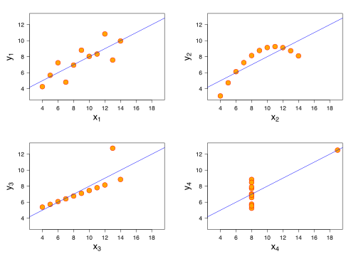
The data sets in the Anscombe's quartet are designed to have approximately the same linear regression line (as well as nearly identical means, standard deviations, and correlations) but are graphically very different. This illustrates the pitfalls of relying solely on a fitted model to understand the relationship between variables.

A fitted linear regression model can be used to identify the relationship between a single predictor variable x_j and the response variable y when all the other predictor variables in the model are "held fixed". Specifically, the interpretation of β_j is the expected change in y for a one-unit change in x_j when the other covariates are held fixed—that is, the expected value of the partial derivative of y with respect to x_j. This is sometimes called the unique effect of x_j on y. In contrast, the marginal effect of x_j on y can be assessed using a correlation coefficient or simple linear regression model relating only x_j to y; this effect is the total derivative of y with respect to x_j.

Care must be taken when interpreting regression results, as some of the regressors may not allow for marginal changes (such as dummy variables, or the intercept term), while others cannot be held fixed (recall the example from the introduction: it would be impossible to "hold t_i fixed" and at the same time change the value of t_i²).

It is possible that the unique effect be nearly zero even when the marginal effect is large. This may imply that some other covariate captures all the information in x_j, so that once that variable is in the model, there is no contribution of x_j to the variation in y. Conversely, the unique effect of x_j can be large while its marginal effect is nearly zero. This would happen if the other covariates explained a great deal of the variation of y, but they mainly explain variation in a way that is complementary to what is captured by x_j. In this case, including the other variables in the model reduces the part of the variability of y that is unrelated to x_j, thereby strengthening the apparent relationship with x_j.

The meaning of the expression "held fixed" may depend on how the values of the predictor variables arise. If the experimenter directly sets the values of the predictor variables according to a study design, the comparisons of interest may literally correspond to comparisons among units whose predictor variables have been "held fixed" by the experimenter. Alternatively, the expression "held fixed" can refer to a selection that takes place in the context of data analysis. In this case, we "hold a variable fixed" by restricting our attention to the subsets of the data that happen to have a common value for the given predictor variable. This is the only interpretation of "held fixed" that can be used in an observational study.

The notion of a "unique effect" is appealing when studying a complex system where multiple interrelated components influence the response variable. In some cases, it can literally be interpreted as the causal effect of an intervention that is linked to the value of a predictor variable. However, it has been argued that in many cases multiple regression analysis fails to clarify the relationships between the predictor variables and the response variable when the predictors are correlated with each other and are not assigned following a study design. ^[9]

Extensions

Numerous extensions of linear regression have been developed, which allow some or all of the assumptions underlying the basic model to be relaxed.

Simple and multiple linear regression

Example of simple linear regression, which has one independent variable

The simplest case of a single scalar predictor variable x and a single scalar response variable y is known as simple linear regression . The extension to multiple and/or vector-valued predictor variables (denoted with a capital X) is known as multiple linear regression, also known as multivariable linear regression (not to be confused with multivariate linear regression ). ^[10]

Multiple linear regression is a generalization of simple linear regression to the case of more than one independent variable, and a special case of general linear models, restricted to one dependent variable. The basic model for multiple linear regression is

${\displaystyle Y_{i}=\beta _{0}+\beta _{1}X_{i1}+\beta _{2}X_{i2}+\ldots +\beta _{p}X_{ip}+\epsilon _{i}}$

for each observation ${\textstyle i=1,\ldots ,n}$.

In the formula above we consider n observations of one dependent variable and p independent variables. Thus, Y_i is the i^th observation of the dependent variable, X_ij is i^th observation of the j^th independent variable, j = 1, 2, ..., p. The values β_j represent parameters to be estimated, and ε_i is the i^th independent identically distributed normal error.

In the more general multivariate linear regression, there is one equation of the above form for each of m > 1 dependent variables that share the same set of explanatory variables and hence are estimated simultaneously with each other:

${\displaystyle Y_{ij}=\beta _{0j}+\beta _{1j}X_{i1}+\beta _{2j}X_{i2}+\ldots +\beta _{pj}X_{ip}+\epsilon _{ij}}$

for all observations indexed as i = 1, ... , n and for all dependent variables indexed as j = 1, ... , m.

Nearly all real-world regression models involve multiple predictors, and basic descriptions of linear regression are often phrased in terms of the multiple regression model. Note, however, that in these cases the response variable y is still a scalar. Another term, multivariate linear regression, refers to cases where y is a vector, i.e., the same as general linear regression.

General linear models

The general linear model considers the situation when the response variable is not a scalar (for each observation) but a vector, y_i. Conditional linearity of ${\displaystyle E(\mathbf {y} \mid \mathbf {x} _{i})=\mathbf {x} _{i}^{\mathsf {T}}B}$ is still assumed, with a matrix B replacing the vector β of the classical linear regression model. Multivariate analogues of ordinary least squares (OLS) and generalized least squares (GLS) have been developed. "General linear models" are also called "multivariate linear models". These are not the same as multivariable linear models (also called "multiple linear models").

Heteroscedastic models

Various models have been created that allow for heteroscedasticity, i.e. the errors for different response variables may have different variances. For example, weighted least squares is a method for estimating linear regression models when the response variables may have different error variances, possibly with correlated errors. (See also Weighted linear least squares, and Generalized least squares.) Heteroscedasticity-consistent standard errors is an improved method for use with uncorrelated but potentially heteroscedastic errors.

Generalized linear models

The Generalized linear model (GLM) is a framework for modeling response variables that are bounded or discrete. This is used, for example:

• when modeling positive quantities (e.g. prices or populations) that vary over a large scale—which are better described using a skewed distribution such as the log-normal distribution or Poisson distribution (although GLMs are not used for log-normal data, instead the response variable is simply transformed using the logarithm function);
• when modeling categorical data, such as the choice of a given candidate in an election (which is better described using a Bernoulli distribution/binomial distribution for binary choices, or a categorical distribution/multinomial distribution for multi-way choices), where there are a fixed number of choices that cannot be meaningfully ordered;
• when modeling ordinal data, e.g. ratings on a scale from 0 to 5, where the different outcomes can be ordered but where the quantity itself may not have any absolute meaning (e.g. a rating of 4 may not be "twice as good" in any objective sense as a rating of 2, but simply indicates that it is better than 2 or 3 but not as good as 5).

Generalized linear models allow for an arbitrary link function, g, that relates the mean of the response variable(s) to the predictors: ${\displaystyle E(Y)=g^{-1}(XB)}$. The link function is often related to the distribution of the response, and in particular it typically has the effect of transforming between the ${\displaystyle (-\infty ,\infty )}$ range of the linear predictor and the range of the response variable.

Some common examples of GLMs are:

• Poisson regression for count data.
• Logistic regression and probit regression for binary data.
• Multinomial logistic regression and multinomial probit regression for categorical data.
• Ordered logit and ordered probit regression for ordinal data.

Single index models^{[ clarification needed ]} allow some degree of nonlinearity in the relationship between x and y, while preserving the central role of the linear predictor β′x as in the classical linear regression model. Under certain conditions, simply applying OLS to data from a single-index model will consistently estimate β up to a proportionality constant. ^[11]

Hierarchical linear models

Hierarchical linear models (or multilevel regression) organizes the data into a hierarchy of regressions, for example where A is regressed on B, and B is regressed on C. It is often used where the variables of interest have a natural hierarchical structure such as in educational statistics, where students are nested in classrooms, classrooms are nested in schools, and schools are nested in some administrative grouping, such as a school district. The response variable might be a measure of student achievement such as a test score, and different covariates would be collected at the classroom, school, and school district levels.

Errors-in-variables

Errors-in-variables models (or "measurement error models") extend the traditional linear regression model to allow the predictor variables X to be observed with error. This error causes standard estimators of β to become biased. Generally, the form of bias is an attenuation, meaning that the effects are biased toward zero.

Group effects

Further information: Multicollinearity

In a multiple linear regression model

${\displaystyle y=\beta _{0}+\beta _{1}x_{1}+\cdots +\beta _{p}x_{p}+\varepsilon ,}$

parameter ${\displaystyle \beta _{j}}$ of predictor variable ${\displaystyle x_{j}}$ represents the individual effect of ${\displaystyle x_{j}}$. It has an interpretation as the expected change in the response variable ${\displaystyle y}$ when ${\displaystyle x_{j}}$ increases by one unit with other predictor variables held constant. When ${\displaystyle x_{j}}$ is strongly correlated with other predictor variables, it is improbable that ${\displaystyle x_{j}}$ can increase by one unit with other variables held constant. In this case, the interpretation of ${\displaystyle \beta _{j}}$ becomes problematic as it is based on an improbable condition, and the effect of ${\displaystyle x_{j}}$ cannot be evaluated in isolation.

For a group of predictor variables, say, ${\displaystyle \{x_{1},x_{2},\dots ,x_{q}\}}$, a group effect ${\displaystyle \xi (\mathbf {w} )}$ is defined as a linear combination of their parameters

${\displaystyle \xi (\mathbf {w} )=w_{1}\beta _{1}+w_{2}\beta _{2}+\dots +w_{q}\beta _{q},}$

where ${\displaystyle \mathbf {w} =(w_{1},w_{2},\dots ,w_{q})^{\intercal }}$ is a weight vector satisfying ${\textstyle \sum _{j=1}^{q}|w_{j}|=1}$. Because of the constraint on ${\displaystyle {w_{j}}}$, ${\displaystyle \xi (\mathbf {w} )}$ is also referred to as a normalized group effect. A group effect ${\displaystyle \xi (\mathbf {w} )}$ has an interpretation as the expected change in ${\displaystyle y}$ when variables in the group ${\displaystyle x_{1},x_{2},\dots ,x_{q}}$ change by the amount ${\displaystyle w_{1},w_{2},\dots ,w_{q}}$, respectively, at the same time with other variables (not in the group) held constant. It generalizes the individual effect of a variable to a group of variables in that (${\displaystyle i}$) if ${\displaystyle q=1}$, then the group effect reduces to an individual effect, and (${\displaystyle ii}$) if ${\displaystyle w_{i}=1}$ and ${\displaystyle w_{j}=0}$ for ${\displaystyle j\neq i}$, then the group effect also reduces to an individual effect. A group effect ${\displaystyle \xi (\mathbf {w} )}$ is said to be meaningful if the underlying simultaneous changes of the ${\displaystyle q}$ variables ${\displaystyle (x_{1},x_{2},\dots ,x_{q})^{\intercal }}$ is probable.

Group effects provide a means to study the collective impact of strongly correlated predictor variables in linear regression models. Individual effects of such variables are not well-defined as their parameters do not have good interpretations. Furthermore, when the sample size is not large, none of their parameters can be accurately estimated by the least squares regression due to the multicollinearity problem. Nevertheless, there are meaningful group effects that have good interpretations and can be accurately estimated by the least squares regression. A simple way to identify these meaningful group effects is to use an all positive correlations (APC) arrangement of the strongly correlated variables under which pairwise correlations among these variables are all positive, and standardize all ${\displaystyle p}$ predictor variables in the model so that they all have mean zero and length one. To illustrate this, suppose that ${\displaystyle \{x_{1},x_{2},\dots ,x_{q}\}}$ is a group of strongly correlated variables in an APC arrangement and that they are not strongly correlated with predictor variables outside the group. Let ${\displaystyle y'}$ be the centred ${\displaystyle y}$ and ${\displaystyle x_{j}'}$ be the standardized ${\displaystyle x_{j}}$. Then, the standardized linear regression model is

${\displaystyle y'=\beta _{1}'x_{1}'+\cdots +\beta _{p}'x_{p}'+\varepsilon .}$

Parameters ${\displaystyle \beta _{j}}$ in the original model, including ${\displaystyle \beta _{0}}$, are simple functions of ${\displaystyle \beta _{j}'}$ in the standardized model. The standardization of variables does not change their correlations, so ${\displaystyle \{x_{1}',x_{2}',\dots ,x_{q}'\}}$ is a group of strongly correlated variables in an APC arrangement and they are not strongly correlated with other predictor variables in the standardized model. A group effect of ${\displaystyle \{x_{1}',x_{2}',\dots ,x_{q}'\}}$ is

${\displaystyle \xi '(\mathbf {w} )=w_{1}\beta _{1}'+w_{2}\beta _{2}'+\dots +w_{q}\beta _{q}',}$

and its minimum-variance unbiased linear estimator is

${\displaystyle {\hat {\xi }}'(\mathbf {w} )=w_{1}{\hat {\beta }}_{1}'+w_{2}{\hat {\beta }}_{2}'+\dots +w_{q}{\hat {\beta }}_{q}',}$

where ${\displaystyle {\hat {\beta }}_{j}'}$ is the least squares estimator of ${\displaystyle \beta _{j}'}$. In particular, the average group effect of the ${\displaystyle q}$ standardized variables is

${\displaystyle \xi _{A}={\frac {1}{q}}(\beta _{1}'+\beta _{2}'+\dots +\beta _{q}'),}$

which has an interpretation as the expected change in ${\displaystyle y'}$ when all ${\displaystyle x_{j}'}$ in the strongly correlated group increase by ${\displaystyle (1/q)}$th of a unit at the same time with variables outside the group held constant. With strong positive correlations and in standardized units, variables in the group are approximately equal, so they are likely to increase at the same time and in similar amount. Thus, the average group effect ${\displaystyle \xi _{A}}$ is a meaningful effect. It can be accurately estimated by its minimum-variance unbiased linear estimator ${\textstyle {\hat {\xi }}_{A}={\frac {1}{q}}({\hat {\beta }}_{1}'+{\hat {\beta }}_{2}'+\dots +{\hat {\beta }}_{q}')}$, even when individually none of the ${\displaystyle \beta _{j}'}$ can be accurately estimated by ${\displaystyle {\hat {\beta }}_{j}'}$.

Not all group effects are meaningful or can be accurately estimated. For example, ${\displaystyle \beta _{1}'}$ is a special group effect with weights ${\displaystyle w_{1}=1}$ and ${\displaystyle w_{j}=0}$ for ${\displaystyle j\neq 1}$, but it cannot be accurately estimated by ${\displaystyle {\hat {\beta }}'_{1}}$. It is also not a meaningful effect. In general, for a group of ${\displaystyle q}$ strongly correlated predictor variables in an APC arrangement in the standardized model, group effects whose weight vectors ${\displaystyle \mathbf {w} }$ are at or near the centre of the simplex ${\textstyle \sum _{j=1}^{q}w_{j}=1}$ (${\displaystyle w_{j}\geq 0}$) are meaningful and can be accurately estimated by their minimum-variance unbiased linear estimators. Effects with weight vectors far away from the centre are not meaningful as such weight vectors represent simultaneous changes of the variables that violate the strong positive correlations of the standardized variables in an APC arrangement. As such, they are not probable. These effects also cannot be accurately estimated.

Applications of the group effects include (1) estimation and inference for meaningful group effects on the response variable, (2) testing for "group significance" of the ${\displaystyle q}$ variables via testing ${\displaystyle H_{0}:\xi _{A}=0}$ versus ${\displaystyle H_{1}:\xi _{A}\neq 0}$, and (3) characterizing the region of the predictor variable space over which predictions by the least squares estimated model are accurate.

A group effect of the original variables ${\displaystyle \{x_{1},x_{2},\dots ,x_{q}\}}$ can be expressed as a constant times a group effect of the standardized variables ${\displaystyle \{x_{1}',x_{2}',\dots ,x_{q}'\}}$. The former is meaningful when the latter is. Thus meaningful group effects of the original variables can be found through meaningful group effects of the standardized variables. ^[12]

Others

In Dempster–Shafer theory, or a linear belief function in particular, a linear regression model may be represented as a partially swept matrix, which can be combined with similar matrices representing observations and other assumed normal distributions and state equations. The combination of swept or unswept matrices provides an alternative method for estimating linear regression models.

Estimation methods

A large number of procedures have been developed for parameter estimation and inference in linear regression. These methods differ in computational simplicity of algorithms, presence of a closed-form solution, robustness with respect to heavy-tailed distributions, and theoretical assumptions needed to validate desirable statistical properties such as consistency and asymptotic efficiency.

Some of the more common estimation techniques for linear regression are summarized below.

Least-squares estimation and related techniques

Main article: Linear least squares

Francis Galton's 1886 illustration of the correlation between the heights of adults and their parents. The observation that adult children's heights tended to deviate less from the mean height than their parents suggested the concept of "regression toward the mean", giving regression its name. The "locus of horizontal tangential points" passing through the leftmost and rightmost points on the ellipse (which is a level curve of the bivariate normal distribution estimated from the data) is the OLS estimate of the regression of parents' heights on children's heights, while the "locus of vertical tangential points" is the OLS estimate of the regression of children's heights on parent's heights. The major axis of the ellipse is the TLS estimate.

Assuming that the independent variables are ${\displaystyle {\vec {x_{i}}}=\left[x_{1}^{i},x_{2}^{i},\ldots ,x_{m}^{i}\right]}$ and the model's parameters are ${\displaystyle {\vec {\beta }}=\left[\beta _{0},\beta _{1},\ldots ,\beta _{m}\right]}$, then the model's prediction would be

${\displaystyle y_{i}\approx \beta _{0}+\sum _{j=1}^{m}\beta _{j}\times x_{j}^{i}}$.

If ${\displaystyle {\vec {x_{i}}}}$ is extended to ${\displaystyle {\vec {x_{i}}}=\left[1,x_{1}^{i},x_{2}^{i},\ldots ,x_{m}^{i}\right]}$ then ${\displaystyle y_{i}}$ would become a dot product of the parameter and the independent vectors, i.e.

${\displaystyle y_{i}\approx \sum _{j=0}^{m}\beta _{j}\times x_{j}^{i}={\vec {\beta }}\cdot {\vec {x_{i}}}}$.

In the least-squares setting, the optimum parameter vector is defined as such that minimizes the sum of mean squared loss:

${\displaystyle {\vec {\hat {\beta }}}={\underset {\vec {\beta }}{\mbox{arg min}}}\,L\left(D,{\vec {\beta }}\right)={\underset {\vec {\beta }}{\mbox{arg min}}}\sum _{i=1}^{n}\left({\vec {\beta }}\cdot {\vec {x_{i}}}-y_{i}\right)^{2}}$

Now putting the independent and dependent variables in matrices ${\displaystyle X}$ and ${\displaystyle Y}$ respectively, the loss function can be rewritten as:

${\displaystyle {\begin{aligned}L\left(D,{\vec {\beta }}\right)&=\|X{\vec {\beta }}-Y\|^{2}\\&=\left(X{\vec {\beta }}-Y\right)^{\textsf {T}}\left(X{\vec {\beta }}-Y\right)\\&=Y^{\textsf {T}}Y-Y^{\textsf {T}}X{\vec {\beta }}-{\vec {\beta }}^{\textsf {T}}X^{\textsf {T}}Y+{\vec {\beta }}^{\textsf {T}}X^{\textsf {T}}X{\vec {\beta }}\end{aligned}}}$

As the loss function is convex, the optimum solution lies at gradient zero. The gradient of the loss function is (using Denominator layout convention):

${\displaystyle {\begin{aligned}{\frac {\partial L\left(D,{\vec {\beta }}\right)}{\partial {\vec {\beta }}}}&={\frac {\partial \left(Y^{\textsf {T}}Y-Y^{\textsf {T}}X{\vec {\beta }}-{\vec {\beta }}^{\textsf {T}}X^{\textsf {T}}Y+{\vec {\beta }}^{\textsf {T}}X^{\textsf {T}}X{\vec {\beta }}\right)}{\partial {\vec {\beta }}}}\\&=-2X^{\textsf {T}}Y+2X^{\textsf {T}}X{\vec {\beta }}\end{aligned}}}$

Setting the gradient to zero produces the optimum parameter:

${\displaystyle {\begin{aligned}-2X^{\textsf {T}}Y+2X^{\textsf {T}}X{\vec {\beta }}&=0\\\Rightarrow X^{\textsf {T}}X{\vec {\beta }}&=X^{\textsf {T}}Y\\\Rightarrow {\vec {\hat {\beta }}}&=\left(X^{\textsf {T}}X\right)^{-1}X^{\textsf {T}}Y\end{aligned}}}$

Note: The ${\displaystyle {\hat {\beta }}}$ obtained may indeed be the local minimum, one needs to differentiate once more to obtain the Hessian matrix and show that it is positive definite. This is provided by the Gauss–Markov theorem.

Linear least squares methods include mainly:

• Ordinary least squares
• Weighted least squares
• Generalized least squares
• Linear Template Fit ^[14]

Maximum-likelihood estimation and related techniques

Maximum likelihood estimation

Maximum likelihood estimation can be performed when the distribution of the error terms is known to belong to a certain parametric family ƒ_θ of probability distributions. ^[15] When f_θ is a normal distribution with zero mean and variance θ, the resulting estimate is identical to the OLS estimate. GLS estimates are maximum likelihood estimates when ε follows a multivariate normal distribution with a known covariance matrix. Let's denote each data point by ${\displaystyle ({\vec {x_{i}}},y_{i})}$ and the regression parameters as ${\displaystyle {\vec {\beta }}}$, and the set of all data by ${\displaystyle D}$ and the cost function by ${\displaystyle L(D,{\vec {\beta }})=\sum _{i}(y_{i}-{\vec {\beta }}\,\cdot \,{\vec {x_{i}}})^{2}}$.

As shown below the same optimal parameter that minimizes ${\displaystyle L(D,{\vec {\beta }})}$ achieves maximum likelihood too. ^[16] Here the assumption is that the dependent variable ${\displaystyle y}$ is a random variable that follows a Gaussian distribution, where the standard deviation is fixed and the mean is a linear combination of ${\displaystyle {\vec {x}}}$:${\displaystyle {\begin{aligned}H(D,{\vec {\beta }})&=\prod _{i=1}^{n}Pr(y_{i}|{\vec {x_{i}}}\,\,;{\vec {\beta }},\sigma )\\&=\prod _{i=1}^{n}{\frac {1}{{\sqrt {2\pi }}\sigma }}\exp \left(-{\frac {\left(y_{i}-{\vec {\beta }}\,\cdot \,{\vec {x_{i}}}\right)^{2}}{2\sigma ^{2}}}\right)\end{aligned}}}$

Now, we need to look for a parameter that maximizes this likelihood function. Since the logarithmic function is strictly increasing, instead of maximizing this function, we can also maximize its logarithm and find the optimal parameter that way. ^[16]

${\displaystyle {\begin{aligned}I(D,{\vec {\beta }})&=\log \prod _{i=1}^{n}Pr(y_{i}|{\vec {x_{i}}}\,\,;{\vec {\beta }},\sigma )\\&=\log \prod _{i=1}^{n}{\frac {1}{{\sqrt {2\pi }}\sigma }}\exp \left(-{\frac {\left(y_{i}-{\vec {\beta }}\,\cdot \,{\vec {x_{i}}}\right)^{2}}{2\sigma ^{2}}}\right)\\&=n\log {\frac {1}{{\sqrt {2\pi }}\sigma }}-{\frac {1}{2\sigma ^{2}}}\sum _{i=1}^{n}\left(y_{i}-{\vec {\beta }}\,\cdot \,{\vec {x_{i}}}\right)^{2}\end{aligned}}}$

The optimal parameter is thus equal to: ^[16]

${\displaystyle {\begin{aligned}{\underset {\vec {\beta }}{\mbox{arg max}}}\,I(D,{\vec {\beta }})&={\underset {\vec {\beta }}{\mbox{arg max}}}\left(n\log {\frac {1}{{\sqrt {2\pi }}\sigma }}-{\frac {1}{2\sigma ^{2}}}\sum _{i=1}^{n}\left(y_{i}-{\vec {\beta }}\,\cdot \,{\vec {x_{i}}}\right)^{2}\right)\\&={\underset {\vec {\beta }}{\mbox{arg min}}}\sum _{i=1}^{n}\left(y_{i}-{\vec {\beta }}\,\cdot \,{\vec {x_{i}}}\right)^{2}\\&={\underset {\vec {\beta }}{\mbox{arg min}}}\,L(D,{\vec {\beta }})\\&={\vec {\hat {\beta }}}\end{aligned}}}$

In this way, the parameter that maximizes ${\displaystyle H(D,{\vec {\beta }})}$ is the same as the one that minimizes ${\displaystyle L(D,{\vec {\beta }})}$. This means that in linear regression, the result of the least squares method is the same as the result of the maximum likelihood estimation method. ^[16]

Regularized Regression

Ridge regression ^{[17] [18] [19]} and other forms of penalized estimation, such as Lasso regression, ^[5] deliberately introduce bias into the estimation of β in order to reduce the variability of the estimate. The resulting estimates generally have lower mean squared error than the OLS estimates, particularly when multicollinearity is present or when overfitting is a problem. They are generally used when the goal is to predict the value of the response variable y for values of the predictors x that have not yet been observed. These methods are not as commonly used when the goal is inference, since it is difficult to account for the bias.

Least Absolute Deviation

Least absolute deviation (LAD) regression is a robust estimation technique in that it is less sensitive to the presence of outliers than OLS (but is less efficient than OLS when no outliers are present). It is equivalent to maximum likelihood estimation under a Laplace distribution model for ε. ^[20]

Adaptive Estimation

If we assume that error terms are independent of the regressors, ${\displaystyle \varepsilon _{i}\perp \mathbf {x} _{i}}$, then the optimal estimator is the 2-step MLE, where the first step is used to non-parametrically estimate the distribution of the error term. ^[21]

Other estimation techniques

Comparison of the Theil–Sen estimator (black) and simple linear regression (blue) for a set of points with outliers

• Bayesian linear regression applies the framework of Bayesian statistics to linear regression. (See also Bayesian multivariate linear regression.) In particular, the regression coefficients β are assumed to be random variables with a specified prior distribution. The prior distribution can bias the solutions for the regression coefficients, in a way similar to (but more general than) ridge regression or lasso regression. In addition, the Bayesian estimation process produces not a single point estimate for the "best" values of the regression coefficients but an entire posterior distribution, completely describing the uncertainty surrounding the quantity. This can be used to estimate the "best" coefficients using the mean, mode, median, any quantile (see quantile regression), or any other function of the posterior distribution.
• Quantile regression focuses on the conditional quantiles of y given X rather than the conditional mean of y given X. Linear quantile regression models a particular conditional quantile, for example the conditional median, as a linear function β^Tx of the predictors.
• Mixed models are widely used to analyze linear regression relationships involving dependent data when the dependencies have a known structure. Common applications of mixed models include analysis of data involving repeated measurements, such as longitudinal data, or data obtained from cluster sampling. They are generally fit as parametric models, using maximum likelihood or Bayesian estimation. In the case where the errors are modeled as normal random variables, there is a close connection between mixed models and generalized least squares. ^[22] Fixed effects estimation is an alternative approach to analyzing this type of data.
• Principal component regression (PCR) ^{[7] [8]} is used when the number of predictor variables is large, or when strong correlations exist among the predictor variables. This two-stage procedure first reduces the predictor variables using principal component analysis, and then uses the reduced variables in an OLS regression fit. While it often works well in practice, there is no general theoretical reason that the most informative linear function of the predictor variables should lie among the dominant principal components of the multivariate distribution of the predictor variables. The partial least squares regression is the extension of the PCR method which does not suffer from the mentioned deficiency.
• Least-angle regression ^[6] is an estimation procedure for linear regression models that was developed to handle high-dimensional covariate vectors, potentially with more covariates than observations.
• The Theil–Sen estimator is a simple robust estimation technique that chooses the slope of the fit line to be the median of the slopes of the lines through pairs of sample points. It has similar statistical efficiency properties to simple linear regression but is much less sensitive to outliers. ^[23]
• Other robust estimation techniques, including the α-trimmed mean approach, and L-, M-, S-, and R-estimators have been introduced.

Applications

See also: Linear least squares § Applications

Linear regression is widely used in biological, behavioral and social sciences to describe possible relationships between variables. It ranks as one of the most important tools used in these disciplines.

Trend line

Main article: Trend estimation

A trend line represents a trend, the long-term movement in time series data after other components have been accounted for. It tells whether a particular data set (say GDP, oil prices or stock prices) have increased or decreased over the period of time. A trend line could simply be drawn by eye through a set of data points, but more properly their position and slope is calculated using statistical techniques like linear regression. Trend lines typically are straight lines, although some variations use higher degree polynomials depending on the degree of curvature desired in the line.

Trend lines are sometimes used in business analytics to show changes in data over time. This has the advantage of being simple. Trend lines are often used to argue that a particular action or event (such as training, or an advertising campaign) caused observed changes at a point in time. This is a simple technique, and does not require a control group, experimental design, or a sophisticated analysis technique. However, it suffers from a lack of scientific validity in cases where other potential changes can affect the data.

Epidemiology

Early evidence relating tobacco smoking to mortality and morbidity came from observational studies employing regression analysis. In order to reduce spurious correlations when analyzing observational data, researchers usually include several variables in their regression models in addition to the variable of primary interest. For example, in a regression model in which cigarette smoking is the independent variable of primary interest and the dependent variable is lifespan measured in years, researchers might include education and income as additional independent variables, to ensure that any observed effect of smoking on lifespan is not due to those other socio-economic factors. However, it is never possible to include all possible confounding variables in an empirical analysis. For example, a hypothetical gene might increase mortality and also cause people to smoke more. For this reason, randomized controlled trials are often able to generate more compelling evidence of causal relationships than can be obtained using regression analyses of observational data. When controlled experiments are not feasible, variants of regression analysis such as instrumental variables regression may be used to attempt to estimate causal relationships from observational data.

Finance

The capital asset pricing model uses linear regression as well as the concept of beta for analyzing and quantifying the systematic risk of an investment. This comes directly from the beta coefficient of the linear regression model that relates the return on the investment to the return on all risky assets.

Economics

Main article: Econometrics

Linear regression is the predominant empirical tool in economics. For example, it is used to predict consumption spending, ^[24] fixed investment spending, inventory investment, purchases of a country's exports, ^[25] spending on imports, ^[25] the demand to hold liquid assets, ^[26] labor demand, ^[27] and labor supply. ^[27]

Environmental science

Linear regression finds application in a wide range of environmental science applications such as land use, ^[28] infectious diseases, ^[29] and air pollution. ^[30] For example, linear regression can be used to predict the changing effects of car pollution. ^[31] One notable example of this application in infectious diseases is the flattening the curve strategy emphasized early in the COVID-19 pandemic, where public health officials dealt with sparse data on infected individuals and sophisticated models of disease transmission to characterize the spread of COVID-19. ^[32]

Building science

Linear regression is commonly used in building science field studies to derive characteristics of building occupants. In a thermal comfort field study, building scientists usually ask occupants' thermal sensation votes, which range from -3 (feeling cold) to 0 (neutral) to +3 (feeling hot), and measure occupants' surrounding temperature data. A neutral or comfort temperature can be calculated based on a linear regression between the thermal sensation vote and indoor temperature, and setting the thermal sensation vote as zero. However, there has been a debate on the regression direction: regressing thermal sensation votes (y-axis) against indoor temperature (x-axis) or the opposite: regressing indoor temperature (y-axis) against thermal sensation votes (x-axis). ^[33]

Machine learning

Linear regression plays an important role in the subfield of artificial intelligence known as machine learning. The linear regression algorithm is one of the fundamental supervised machine-learning algorithms due to its relative simplicity and well-known properties. ^[34]

History

Least squares linear regression, as a means of finding a good rough linear fit to a set of points was performed by Legendre (1805) and Gauss (1809) for the prediction of planetary movement. Quetelet was responsible for making the procedure well-known and for using it extensively in the social sciences. ^[35]

See also

• Mathematics portal

• Analysis of variance
• Blinder–Oaxaca decomposition
• Censored regression model
• Cross-sectional regression
• Curve fitting
• Empirical Bayes method
• Errors and residuals
• Lack-of-fit sum of squares
• Line fitting
• Linear classifier
• Linear equation
• Logistic regression
• M-estimator
• Multivariate adaptive regression spline
• Nonlinear regression
• Nonparametric regression
• Normal equations
• Projection pursuit regression
• Response modeling methodology
• Segmented linear regression
• Standard deviation line
• Stepwise regression
• Structural break
• Support vector machine
• Truncated regression model
• Deming regression

References

Citations

1. Freedman, David A. (2009). Statistical Models: Theory and Practice. Cambridge University Press. p. 26. A simple regression equation has on the right hand side an intercept and an explanatory variable with a slope coefficient. A multiple regression e right hand side, each with its own slope coefficient
2. Rencher, Alvin C.; Christensen, William F. (2012), "Chapter 10, Multivariate regression – Section 10.1, Introduction", Methods of Multivariate Analysis, Wiley Series in Probability and Statistics, vol. 709 (3rd ed.), John Wiley & Sons, p. 19, ISBN   9781118391679, archived from the original on 2024-10-04, retrieved 2015-02-07.
3. "Linear Regression in Machine learning". GeeksforGeeks. 2018-09-13. Archived from the original on 2024-10-04. Retrieved 2024-08-25.
4. Yan, Xin (2009), Linear Regression Analysis: Theory and Computing, World Scientific, pp. 1–2, ISBN   9789812834119, archived from the original on 2024-10-04, retrieved 2015-02-07, Regression analysis ... is probably one of the oldest topics in mathematical statistics dating back to about two hundred years ago. The earliest form of the linear regression was the least squares method, which was published by Legendre in 1805, and by Gauss in 1809 ... Legendre and Gauss both applied the method to the problem of determining, from astronomical observations, the orbits of bodies about the sun.
5. Tibshirani, Robert (1996). "Regression Shrinkage and Selection via the Lasso". Journal of the Royal Statistical Society, Series B. 58 (1): 267–288. doi:10.1111/j.2517-6161.1996.tb02080.x. JSTOR   2346178.
6. Efron, Bradley; Hastie, Trevor; Johnstone, Iain; Tibshirani, Robert (2004). "Least Angle Regression". The Annals of Statistics. 32 (2): 407–451. arXiv: math/0406456 . doi:10.1214/009053604000000067. JSTOR   3448465. S2CID   204004121.
7. Hawkins, Douglas M. (1973). "On the Investigation of Alternative Regressions by Principal Component Analysis". Journal of the Royal Statistical Society, Series C. 22 (3): 275–286. doi:10.2307/2346776. JSTOR   2346776.
8. Jolliffe, Ian T. (1982). "A Note on the Use of Principal Components in Regression". Journal of the Royal Statistical Society, Series C. 31 (3): 300–303. doi:10.2307/2348005. JSTOR   2348005.
9. Berk, Richard A. (2007). "Regression Analysis: A Constructive Critique". Criminal Justice Review. 32 (3): 301–302. doi:10.1177/0734016807304871. S2CID   145389362.
10. Hidalgo, Bertha; Goodman, Melody (2012-11-15). "Multivariate or Multivariable Regression?". American Journal of Public Health. 103 (1): 39–40. doi:10.2105/AJPH.2012.300897. ISSN   0090-0036. PMC   3518362 . PMID   23153131.
11. Brillinger, David R. (1977). "The Identification of a Particular Nonlinear Time Series System". Biometrika. 64 (3): 509–515. doi:10.1093/biomet/64.3.509. JSTOR   2345326.
12. Tsao, Min (2022). "Group least squares regression for linear models with strongly correlated predictor variables". Annals of the Institute of Statistical Mathematics. 75 (2): 233–250. arXiv: 1804.02499 . doi:10.1007/s10463-022-00841-7. S2CID   237396158.
13. Galton, Francis (1886). "Regression Towards Mediocrity in Hereditary Stature". The Journal of the Anthropological Institute of Great Britain and Ireland. 15: 246–263. doi:10.2307/2841583. ISSN   0959-5295. JSTOR   2841583.
14. Britzger, Daniel (2022). "The Linear Template Fit". Eur. Phys. J. C. 82 (8): 731. arXiv: 2112.01548 . Bibcode:2022EPJC...82..731B. doi:10.1140/epjc/s10052-022-10581-w. S2CID   244896511.
15. Lange, Kenneth L.; Little, Roderick J. A.; Taylor, Jeremy M. G. (1989). "Robust Statistical Modeling Using the t Distribution" (PDF). Journal of the American Statistical Association. 84 (408): 881–896. doi:10.2307/2290063. JSTOR   2290063. Archived (PDF) from the original on 2024-10-04. Retrieved 2019-09-02.
16. Machine learning: a probabilistic perspective Archived 2018-11-04 at the Wayback Machine , Kevin P Murphy, 2012, p. 217, Cambridge, MA
17. Swindel, Benee F. (1981). "Geometry of Ridge Regression Illustrated". The American Statistician. 35 (1): 12–15. doi:10.2307/2683577. JSTOR   2683577.
18. Draper, Norman R.; van Nostrand; R. Craig (1979). "Ridge Regression and James-Stein Estimation: Review and Comments". Technometrics. 21 (4): 451–466. doi:10.2307/1268284. JSTOR   1268284.
19. Hoerl, Arthur E.; Kennard, Robert W.; Hoerl, Roger W. (1985). "Practical Use of Ridge Regression: A Challenge Met". Journal of the Royal Statistical Society, Series C. 34 (2): 114–120. JSTOR   2347363.
20. Narula, Subhash C.; Wellington, John F. (1982). "The Minimum Sum of Absolute Errors Regression: A State of the Art Survey". International Statistical Review. 50 (3): 317–326. doi:10.2307/1402501. JSTOR   1402501.
21. Stone, C. J. (1975). "Adaptive maximum likelihood estimators of a location parameter". The Annals of Statistics. 3 (2): 267–284. doi: 10.1214/aos/1176343056 . JSTOR   2958945.
22. Goldstein, H. (1986). "Multilevel Mixed Linear Model Analysis Using Iterative Generalized Least Squares". Biometrika. 73 (1): 43–56. doi:10.1093/biomet/73.1.43. JSTOR   2336270.
23. Theil, H. (1950). "A rank-invariant method of linear and polynomial regression analysis. I, II, III". Nederl. Akad. Wetensch., Proc. 53: 386–392, 521–525, 1397–1412. MR   0036489.; Sen, Pranab Kumar (1968). "Estimates of the regression coefficient based on Kendall's tau". Journal of the American Statistical Association . 63 (324): 1379–1389. doi:10.2307/2285891. JSTOR   2285891. MR   0258201..
24. Deaton, Angus (1992). Understanding Consumption. Oxford University Press. ISBN   978-0-19-828824-4.
25. Krugman, Paul R.; Obstfeld, M.; Melitz, Marc J. (2012). International Economics: Theory and Policy (9th global ed.). Harlow: Pearson. ISBN   9780273754091.
26. Laidler, David E. W. (1993). The Demand for Money: Theories, Evidence, and Problems (4th ed.). New York: Harper Collins. ISBN   978-0065010985.
27. Ehrenberg; Smith (2008). Modern Labor Economics (10th international ed.). London: Addison-Wesley. ISBN   9780321538963.
28. Hoek, Gerard; Beelen, Rob; de Hoogh, Kees; Vienneau, Danielle; Gulliver, John; Fischer, Paul; Briggs, David (2008-10-01). "A review of land-use regression models to assess spatial variation of outdoor air pollution". Atmospheric Environment. 42 (33): 7561–7578. Bibcode:2008AtmEn..42.7561H. doi:10.1016/j.atmosenv.2008.05.057. ISSN   1352-2310.
29. Imai, Chisato; Hashizume, Masahiro (2015). "A Systematic Review of Methodology: Time Series Regression Analysis for Environmental Factors and Infectious Diseases". Tropical Medicine and Health. 43 (1): 1–9. doi:10.2149/tmh.2014-21. hdl: 10069/35301 . PMC   4361341 . PMID   25859149. Archived from the original on 2024-10-04. Retrieved 2024-02-03.
30. Milionis, A. E.; Davies, T. D. (1994-09-01). "Regression and stochastic models for air pollution—I. Review, comments and suggestions". Atmospheric Environment. 28 (17): 2801–2810. Bibcode:1994AtmEn..28.2801M. doi:10.1016/1352-2310(94)90083-3. ISSN   1352-2310. Archived from the original on 2024-10-04. Retrieved 2024-05-07.
31. Hoffman, Szymon; Filak, Mariusz; Jasiński, Rafal (8 December 2024). "Air Quality Modeling with the Use of Regression Neural Networks". Int J Environ Res Public Health. 19 (24): 16494. doi: 10.3390/ijerph192416494 . PMC   9779138 . PMID   36554373.
32. CDC (2024-10-28). "Behind the Model: CDC's Tools to Assess Epidemic Trends". CFA: Behind the Model. Retrieved 2024-11-14.
33. Sun, Ruiji; Schiavon, Stefano; Brager, Gail; Arens, Edward; Zhang, Hui; Parkinson, Thomas; Zhang, Chenlu (2024). "Causal Thinking: Uncovering Hidden Assumptions and Interpretations of Statistical Analysis in Building Science". Building and Environment. 259. doi: 10.1016/j.buildenv.2024.111530 .
34. "Linear Regression (Machine Learning)" (PDF). University of Pittsburgh. Archived (PDF) from the original on 2017-02-02. Retrieved 2018-06-21.
35. Stigler, Stephen M. (1986). The History of Statistics: The Measurement of Uncertainty before 1900 . Cambridge: Harvard. ISBN   0-674-40340-1.

Sources

• Cohen, J., Cohen P., West, S. G., & Aiken, L. S. (2003). Applied multiple regression/correlation analysis for the behavioral sciences Archived 2024-10-04 at the Wayback Machine . (2nd ed.) Hillsdale, New Jersey: Lawrence Erlbaum Associates
• Charles Darwin. The Variation of Animals and Plants under Domestication. (1868) (Chapter XIII describes what was known about reversion in Galton's time. Darwin uses the term "reversion".)
• Draper, N. R.; Smith, H. (1998). Applied Regression Analysis (3rd ed.). John Wiley. ISBN   978-0-471-17082-2.
• Francis Galton. "Regression Towards Mediocrity in Hereditary Stature," Journal of the Anthropological Institute, 15:246–263 (1886). (Facsimile at: Archived 2016-03-10 at the Wayback Machine )
• Robert S. Pindyck and Daniel L. Rubinfeld (1998, 4th ed.). Econometric Models and Economic Forecasts, ch. 1 (Intro, including appendices on Σ operators & derivation of parameter est.) & Appendix 4.3 (mult. regression in matrix form).

Further reading

• Pedhazur, Elazar J (1982). Multiple regression in behavioral research: Explanation and prediction (2nd ed.). New York: Holt, Rinehart and Winston. ISBN   978-0-03-041760-3.
• Mathieu Rouaud, 2013: Probability, Statistics and Estimation Chapter 2: Linear Regression, Linear Regression with Error Bars and Nonlinear Regression.
• National Physical Laboratory (1961). "Chapter 1: Linear Equations and Matrices: Direct Methods". Modern Computing Methods. Notes on Applied Science. Vol. 16 (2nd ed.). Her Majesty's Stationery Office.

External links

• Least-Squares Regression, PhET Interactive simulations, University of Colorado at Boulder
• DIY Linear Fit