Multivariate adaptive regression spline

In statistics, multivariate adaptive regression splines (MARS) is a form of regression analysis introduced by Jerome H. Friedman in 1991. ^[1] It is a non-parametric regression technique and can be seen as an extension of linear models that automatically models nonlinearities and interactions between variables.

The term "MARS" is trademarked and licensed to Salford Systems. In order to avoid trademark infringements, many open-source implementations of MARS are called "Earth". ^{[2] [3]}

The basics

This section introduces MARS using a few examples. We start with a set of data: a matrix of input variables x, and a vector of the observed responses y, with a response for each row in x. For example, the data could be:

x	y
10.5	16.4
10.7	18.8
10.8	19.7
...	...
20.6	77.0

Here there is only one independent variable, so the x matrix is just a single column. Given these measurements, we would like to build a model which predicts the expected y for a given x.

A linear model

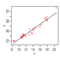
A linear model for the above data is

${\displaystyle {\widehat {y}}=-37+5.1x}$

The hat on the ${\displaystyle {\widehat {y}}}$ indicates that ${\displaystyle {\widehat {y}}}$ is estimated from the data. The figure on the right shows a plot of this function: a line giving the predicted ${\displaystyle {\widehat {y}}}$ versus x, with the original values of y shown as red dots.

The data at the extremes of x indicates that the relationship between y and x may be non-linear (look at the red dots relative to the regression line at low and high values of x). We thus turn to MARS to automatically build a model taking into account non-linearities. MARS software constructs a model from the given x and y as follows

${\displaystyle {\begin{aligned}{\widehat {y}}=&\ 25\\&{}+6.1\max(0,x-13)\\&{}-3.1\max(0,13-x)\end{aligned}}}$

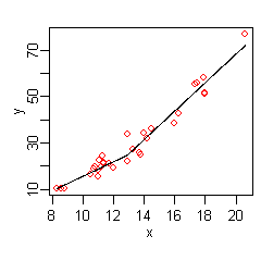
A simple MARS model of the same data

The figure on the right shows a plot of this function: the predicted ${\displaystyle {\widehat {y}}}$ versus x, with the original values of y once again shown as red dots. The predicted response is now a better fit to the original y values.

MARS has automatically produced a kink in the predicted y to take into account non-linearity. The kink is produced by hinge functions. The hinge functions are the expressions starting with ${\displaystyle \max }$ (where ${\displaystyle \max(a,b)}$ is ${\displaystyle a}$ if ${\displaystyle a>b}$, else ${\displaystyle b}$). Hinge functions are described in more detail below.

In this simple example, we can easily see from the plot that y has a non-linear relationship with x (and might perhaps guess that y varies with the square of x). However, in general there will be multiple independent variables, and the relationship between y and these variables will be unclear and not easily visible by plotting. We can use MARS to discover that non-linear relationship.

An example MARS expression with multiple variables is

${\displaystyle {\begin{aligned}\mathrm {ozone} =&\ 5.2\\&{}+0.93\max(0,\mathrm {temp} -58)\\&{}-0.64\max(0,\mathrm {temp} -68)\\&{}-0.046\max(0,234-\mathrm {ibt} )\\&{}-0.016\max(0,\mathrm {wind} -7)\max(0,200-\mathrm {vis} )\end{aligned}}}$

Variable interaction in a MARS model

This expression models air pollution (the ozone level) as a function of the temperature and a few other variables. Note that the last term in the formula (on the last line) incorporates an interaction between ${\displaystyle \mathrm {wind} }$ and ${\displaystyle \mathrm {vis} }$.

The figure on the right plots the predicted ${\displaystyle \mathrm {ozone} }$ as ${\displaystyle \mathrm {wind} }$ and ${\displaystyle \mathrm {vis} }$ vary, with the other variables fixed at their median values. The figure shows that wind does not affect the ozone level unless visibility is low. We see that MARS can build quite flexible regression surfaces by combining hinge functions.

To obtain the above expression, the MARS model building procedure automatically selects which variables to use (some variables are important, others not), the positions of the kinks in the hinge functions, and how the hinge functions are combined.

The MARS model

MARS builds models of the form

${\displaystyle {\widehat {f}}(x)=\sum _{i=1}^{k}c_{i}B_{i}(x).}$

The model is a weighted sum of basis functions ${\displaystyle B_{i}(x)}$. Each ${\displaystyle c_{i}}$ is a constant coefficient. For example, each line in the formula for ozone above is one basis function multiplied by its coefficient.

Each basis function ${\displaystyle B_{i}(x)}$ takes one of the following three forms:

1) a constant 1. There is just one such term, the intercept. In the ozone formula above, the intercept term is 5.2.

2) a hinge function. A hinge function has the form ${\displaystyle \max(0,x-{\text{constant}})}$ or ${\displaystyle \max(0,{\text{constant}}-x)}$. MARS automatically selects variables and values of those variables for knots of the hinge functions. Examples of such basis functions can be seen in the middle three lines of the ozone formula.

3) a product of two or more hinge functions. These basis functions can model interaction between two or more variables. An example is the last line of the ozone formula.

Hinge functions

A mirrored pair of hinge functions with a knot at x=3.1

Further information: Hinge function

A key part of MARS models are hinge functions taking the form

${\displaystyle \max(0,x-c)}$

or

${\displaystyle \max(0,c-x)}$

where ${\displaystyle c}$ is a constant, called the knot. The figure on the right shows a mirrored pair of hinge functions with a knot at 3.1.

A hinge function is zero for part of its range, so can be used to partition the data into disjoint regions, each of which can be treated independently. Thus for example a mirrored pair of hinge functions in the expression

${\displaystyle 6.1\max(0,x-13)-3.1\max(0,13-x)}$

creates the piecewise linear graph shown for the simple MARS model in the previous section.

One might assume that only piecewise linear functions can be formed from hinge functions, but hinge functions can be multiplied together to form non-linear functions.

Hinge functions are also called ramp, hockey stick, or rectifier functions. Instead of the ${\displaystyle \max }$ notation used in this article, hinge functions are often represented by ${\displaystyle [\pm (x_{i}-c)]_{+}}$ where ${\displaystyle [\cdot ]_{+}}$ means take the positive part.

The model building process

See also: Stepwise regression

MARS builds a model in two phases: the forward and the backward pass. This two-stage approach is the same as that used by recursive partitioning trees.

The forward pass

MARS starts with a model which consists of just the intercept term (which is the mean of the response values).

MARS then repeatedly adds basis function in pairs to the model. At each step it finds the pair of basis functions that gives the maximum reduction in sum-of-squares residual error (it is a greedy algorithm). The two basis functions in the pair are identical except that a different side of a mirrored hinge function is used for each function. Each new basis function consists of a term already in the model (which could perhaps be the intercept term) multiplied by a new hinge function. A hinge function is defined by a variable and a knot, so to add a new basis function, MARS must search over all combinations of the following:

1) existing terms (called parent terms in this context)

2) all variables (to select one for the new basis function)

3) all values of each variable (for the knot of the new hinge function).

To calculate the coefficient of each term, MARS applies a linear regression over the terms.

This process of adding terms continues until the change in residual error is too small to continue or until the maximum number of terms is reached. The maximum number of terms is specified by the user before model building starts.

The search at each step is usually done in a brute-force fashion, but a key aspect of MARS is that because of the nature of hinge functions, the search can be done quickly using a fast least-squares update technique. Brute-force search can be sped up by using a heuristic that reduces the number of parent terms considered at each step ("Fast MARS" ^[4] ).

The backward pass

The forward pass usually overfits the model. To build a model with better generalization ability, the backward pass prunes the model, deleting the least effective term at each step until it finds the best submodel. Model subsets are compared using the Generalized cross validation (GCV) criterion described below.

The backward pass has an advantage over the forward pass: at any step it can choose any term to delete, whereas the forward pass at each step can only see the next pair of terms.

The forward pass adds terms in pairs, but the backward pass typically discards one side of the pair and so terms are often not seen in pairs in the final model. A paired hinge can be seen in the equation for ${\displaystyle {\widehat {y}}}$ in the first MARS example above; there are no complete pairs retained in the ozone example.

Generalized cross validation

Further information: Cross-validation (statistics), Model selection, and Akaike information criterion

The backward pass compares the performance of different models using Generalized Cross-Validation (GCV), a minor variant on the Akaike information criterion that approximates the leave-one-out cross-validation score in the special case where errors are Gaussian, or where the squared error loss function is used. GCV was introduced by Craven and Wahba and extended by Friedman for MARS; lower values of GCV indicate better models. The formula for the GCV is

GCV = RSS / (N · (1 − (effective number of parameters) / N)²)

where RSS is the residual sum-of-squares measured on the training data and N is the number of observations (the number of rows in the x matrix).

The effective number of parameters is defined as

(effective number of parameters) = (number of mars terms) + (penalty) · ((number of Mars terms) − 1 ) / 2

where penalty is typically 2 (giving results equivalent to the Akaike information criterion) but can be increased by the user if they so desire.

Note that

(number of Mars terms − 1 ) / 2

is the number of hinge-function knots, so the formula penalizes the addition of knots. Thus the GCV formula adjusts (i.e. increases) the training RSS to penalize more complex models. We penalize flexibility because models that are too flexible will model the specific realization of noise in the data instead of just the systematic structure of the data.

Constraints

One constraint has already been mentioned: the user can specify the maximum number of terms in the forward pass.

A further constraint can be placed on the forward pass by specifying a maximum allowable degree of interaction. Typically only one or two degrees of interaction are allowed, but higher degrees can be used when the data warrants it. The maximum degree of interaction in the first MARS example above is one (i.e. no interactions or an additive model); in the ozone example it is two.

Other constraints on the forward pass are possible. For example, the user can specify that interactions are allowed only for certain input variables. Such constraints could make sense because of knowledge of the process that generated the data.

Pros and cons

No regression modeling technique is best for all situations. The guidelines below are intended to give an idea of the pros and cons of MARS, but there will be exceptions to the guidelines. It is useful to compare MARS to recursive partitioning and this is done below. (Recursive partitioning is also commonly called regression trees, decision trees, or CART; see the recursive partitioning article for details).

• MARS models are more flexible than linear regression models.
• MARS models are simple to understand and interpret. ^[5] Compare the equation for ozone concentration above to, say, the innards of a trained neural network or a random forest.
• MARS can handle both continuous and categorical data. ^{[6] [7]} MARS tends to be better than recursive partitioning for numeric data because hinges are more appropriate for numeric variables than the piecewise constant segmentation used by recursive partitioning.
• Building MARS models often requires little or no data preparation. ^[5] The hinge functions automatically partition the input data, so the effect of outliers is contained. In this respect MARS is similar to recursive partitioning which also partitions the data into disjoint regions, although using a different method.
• MARS (like recursive partitioning) does automatic variable selection (meaning it includes important variables in the model and excludes unimportant ones). However, there can be some arbitrariness in the selection, especially when there are correlated predictors, and this can affect interpretability. ^[5]
• MARS models tend to have a good bias-variance trade-off. The models are flexible enough to model non-linearity and variable interactions (thus MARS models have fairly low bias), yet the constrained form of MARS basis functions prevents too much flexibility (thus MARS models have fairly low variance).
• MARS is suitable for handling large datasets, and implementations run very quickly. However, recursive partitioning can be faster than MARS^{[ citation needed ]}.
• With MARS models, as with any non-parametric regression, parameter confidence intervals and other checks on the model cannot be calculated directly (unlike linear regression models). Cross-validation and related techniques must be used for validating the model instead.
• The earth, mda, and polspline implementations do not allow missing values in predictors, but free implementations of regression trees (such as rpart and party) do allow missing values using a technique called surrogate splits.
• MARS models can make predictions very quickly, as they only require evaluating a linear function of the predictors.
• The resulting fitted function is continuous, unlike recursive partitioning, which can give a more realistic model in some situations. (However, the model is not smooth or differentiable).

Extensions and related concepts

• Generalized linear models (GLMs) can be incorporated into MARS models by applying a link function after the MARS model is built. Thus, for example, MARS models can incorporate logistic regression to predict probabilities.
• Non-linear regression is used when the underlying form of the function is known and regression is used only to estimate the parameters of that function. MARS, on the other hand, estimates the functions themselves, albeit with severe constraints on the nature of the functions. (These constraints are necessary because discovering a model from the data is an inverse problem that is not well-posed without constraints on the model.)
• Recursive partitioning (commonly called CART). MARS can be seen as a generalization of recursive partitioning that allows for continuous models, which can provide a better fit for numerical data.
• Generalized additive models. Unlike MARS, GAMs fit smooth loess or polynomial splines rather than hinge functions, and they do not automatically model variable interactions. The smoother fit and lack of regression terms reduces variance when compared to MARS, but ignoring variable interactions can worsen the bias.
• TSMARS. Time Series Mars is the term used when MARS models are applied in a time series context. Typically in this set up the predictors are the lagged time series values resulting in autoregressive spline models. These models and extensions to include moving average spline models are described in "Univariate Time Series Modelling and Forecasting using TSMARS: A study of threshold time series autoregressive, seasonal and moving average models using TSMARS".
• Bayesian MARS (BMARS) uses the same model form, but builds the model using a Bayesian approach. It may arrive at different optimal MARS models because the model building approach is different. The result of BMARS is typically an ensemble of posterior samples of MARS models, which allows for probabilistic prediction. ^[8]

See also

• Linear regression
• Local regression
• Rational function modeling
• Segmented regression
• Spline interpolation
• Spline regression

References

1. Friedman, J. H. (1991). "Multivariate Adaptive Regression Splines". The Annals of Statistics. 19 (1): 1–67. CiteSeerX   10.1.1.382.970 . doi:10.1214/aos/1176347963. JSTOR   2241837. MR   1091842. Zbl   0765.62064.
2. CRAN Package earth
3. Earth – Multivariate adaptive regression splines in Orange (Python machine learning library)
4. Friedman, J. H. (1993) Fast MARS, Stanford University Department of Statistics, Technical Report 110
5. Kuhn, Max; Johnson, Kjell (2013). Applied Predictive Modeling. New York, NY: Springer New York. doi:10.1007/978-1-4614-6849-3. ISBN   9781461468486.
6. Friedman, Jerome H. (1993). "Estimating Functions of Mixed Ordinal and Categorical Variables Using Adaptive Splines". In Stephan Morgenthaler; Elvezio Ronchetti; Werner Stahel (eds.). New Directions in Statistical Data Analysis and Robustness. Birkhauser.
7. Friedman, Jerome H. (1991-06-01). "Estimating Functions of Mixed Ordinal and Categorical Variables Using Adaptive Splines". DTIC. Archived from the original on April 11, 2022. Retrieved 2022-04-11.
8. Denison, D. G. T.; Mallick, B. K.; Smith, A. F. M. (1 December 1998). "Bayesian MARS" (PDF). Statistics and Computing. 8 (4): 337–346. doi:10.1023/A:1008824606259. ISSN   1573-1375. S2CID   12570055.

Further reading

• Hastie T., Tibshirani R., and Friedman J.H. (2009) The Elements of Statistical Learning, 2nd edition. Springer, ISBN   978-0-387-84857-0 (has a section on MARS)
• Faraway J. (2005) Extending the Linear Model with R, CRC, ISBN   978-1-58488-424-8 (has an example using MARS with R)
• Heping Zhang and Burton H. Singer (2010) Recursive Partitioning and Applications, 2nd edition. Springer, ISBN   978-1-4419-6823-4 (has a chapter on MARS and discusses some tweaks to the algorithm)
• Denison D.G.T., Holmes C.C., Mallick B.K., and Smith A.F.M. (2004) Bayesian Methods for Nonlinear Classification and Regression, Wiley, ISBN   978-0-471-49036-4
• Berk R.A. (2008) Statistical learning from a regression perspective, Springer, ISBN   978-0-387-77500-5

External links

Several free and commercial software packages are available for fitting MARS-type models.

Free software

• R packages:
  • earth function in the earth package
  • mars function in the mda package
  • polymars function in the polspline package. Not Friedman's MARS.
  • bass function in the BASS package for Bayesian MARS.
• Matlab code:
  • ARESLab: Adaptive Regression Splines toolbox for Matlab
  • Code from the book Bayesian Methods for Nonlinear Classification and Regression ^[1] for Bayesian MARS.
• Python
  • Earth – Multivariate adaptive regression splines
  • py-earth
  • pyBASS for Bayesian MARS.

Commercial software

• MARS from Salford Systems. Based on Friedman's implementation.
• STATISTICA Data Miner from StatSoft
• ADAPTIVEREG from SAS.

1. Denison, D. G. T.; Holmes, C. C.; Mallick, B. K.; Smith, A. F. M. (2002). Bayesian methods for nonlinear classification and regression. Chichester, England: Wiley. ISBN   978-0-471-49036-4.