Moment (mathematics)

For the physical concept, see Moment (physics).

In mathematics, the moments of a function are certain quantitative measures related to the shape of the function's graph. If the function represents mass density, then the zeroth moment is the total mass, the first moment (normalized by total mass) is the center of mass, and the second moment is the moment of inertia. If the function is a probability distribution, then the first moment is the expected value, the second central moment is the variance, the third standardized moment is the skewness, and the fourth standardized moment is the kurtosis.

For a distribution of mass or probability on a bounded interval, the collection of all the moments (of all orders, from 0 to ∞) uniquely determines the distribution (Hausdorff moment problem). The same is not true on unbounded intervals (Hamburger moment problem).

In the mid-nineteenth century, Pafnuty Chebyshev became the first person to think systematically in terms of the moments of random variables. ^[1]

Significance of the moments

The n-th raw moment (i.e., moment about zero) of a random variable ${\displaystyle X}$ with density function ${\displaystyle f(x)}$ is defined by ^[2] $${\displaystyle \mu '_{n}=\langle X^{n}\rangle ~{\overset {\mathrm {def} }{=}}~{\begin{cases}\sum _{i}x_{i}^{n}f(x_{i}),&{\text{discrete distribution}}\\[1.2ex]\int x^{n}f(x)\,dx,&{\text{continuous distribution}}\end{cases}}}$$The n-th moment of a real-valued continuous random variable with density function ${\displaystyle f(x)}$ about a value ${\displaystyle c}$ is the integral $${\displaystyle \mu _{n}=\int _{-\infty }^{\infty }(x-c)^{n}\,f(x)\,\mathrm {d} x.}$$

It is possible to define moments for random variables in a more general fashion than moments for real-valued functions — see moments in metric spaces. The moment of a function, without further explanation, usually refers to the above expression with ${\displaystyle c=0}$. For the second and higher moments, the central moment (moments about the mean, with c being the mean) are usually used rather than the moments about zero, because they provide clearer information about the distribution's shape.

Other moments may also be defined. For example, the nth inverse moment about zero is ${\displaystyle \operatorname {E} \left[X^{-n}\right]}$ and the n-th logarithmic moment about zero is ${\displaystyle \operatorname {E} \left[\ln ^{n}(X)\right].}$

The n-th moment about zero of a probability density function ${\displaystyle f(x)}$ is the expected value of ${\displaystyle X^{n}}$ and is called a raw moment or crude moment. ^[3] The moments about its mean ${\displaystyle \mu }$ are called central moments; these describe the shape of the function, independently of translation.

If ${\displaystyle f}$ is a probability density function, then the value of the integral above is called the n-th moment of the probability distribution. More generally, if F is a cumulative probability distribution function of any probability distribution, which may not have a density function, then the n-th moment of the probability distribution is given by the Riemann–Stieltjes integral $${\displaystyle \mu '_{n}=\operatorname {E} \left[X^{n}\right]=\int _{-\infty }^{\infty }x^{n}\,\mathrm {d} F(x)}$$where X is a random variable that has this cumulative distribution F, and E is the expectation operator or mean. When$${\displaystyle \operatorname {E} \left[\left|X^{n}\right|\right]=\int _{-\infty }^{\infty }\left|x^{n}\right|\,\mathrm {d} F(x)=\infty }$$the moment is said not to exist. If the n-th moment about any point exists, so does the (n − 1)-th moment (and thus, all lower-order moments) about every point. The zeroth moment of any probability density function is 1, since the area under any probability density function must be equal to one.

Significance of moments (raw, central, standardised) and cumulants (raw, normalised), in connection with named properties of distributions

Moment ordinal	Moment			Cumulant
	Raw	Central	Standardized	Raw	Normalized
1	Mean	0	0	Mean	—
2	–	Variance	1	Variance	1
3	–	–	Skewness	–	Skewness
4	–	–	(Non-excess or historical) kurtosis	–	Excess kurtosis
5	–	–	Hyperskewness	–	–
6	–	–	Hypertailedness	–	–
7+	–	–	–	–	–

Standardized moments

Main article: Standardized moment

The normalisedn-th central moment or standardised moment is the n-th central moment divided by σⁿ; the normalised n-th central moment of the random variable X is $${\displaystyle {\frac {\mu _{n}}{\sigma ^{n}}}={\frac {\operatorname {E} \left[(X-\mu )^{n}\right]}{\sigma ^{n}}}={\frac {\operatorname {E} \left[(X-\mu )^{n}\right]}{\operatorname {E} \left[(X-\mu )^{2}\right]^{\frac {n}{2}}}}.}$$

These normalised central moments are dimensionless quantities, which represent the distribution independently of any linear change of scale.

Notable moments

Mean

Main article: Mean

The first raw moment is the mean, usually denoted ${\displaystyle \mu \equiv \operatorname {E} [X].}$

Variance

Main article: Variance

The second central moment is the variance. The positive square root of the variance is the standard deviation ${\displaystyle \sigma \equiv \left(\operatorname {E} \left[(x-\mu )^{2}\right]\right)^{\frac {1}{2}}.}$

Skewness

Main article: Skewness

The third central moment is the measure of the lopsidedness of the distribution; any symmetric distribution will have a third central moment, if defined, of zero. The normalised third central moment is called the skewness, often γ. A distribution that is skewed to the left (the tail of the distribution is longer on the left) will have a negative skewness. A distribution that is skewed to the right (the tail of the distribution is longer on the right), will have a positive skewness.

For distributions that are not too different from the normal distribution, the median will be somewhere near μ − γσ/6; the mode about μ − γσ/2.

Kurtosis

Main article: Kurtosis

The fourth central moment is a measure of the heaviness of the tail of the distribution. Since it is the expectation of a fourth power, the fourth central moment, where defined, is always nonnegative; and except for a point distribution, it is always strictly positive. The fourth central moment of a normal distribution is 3σ⁴.

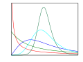
The kurtosis κ is defined to be the standardized fourth central moment. (Equivalently, as in the next section, excess kurtosis is the fourth cumulant divided by the square of the second cumulant.) ^{[4] [5]} If a distribution has heavy tails, the kurtosis will be high (sometimes called leptokurtic); conversely, light-tailed distributions (for example, bounded distributions such as the uniform) have low kurtosis (sometimes called platykurtic).

The kurtosis can be positive without limit, but κ must be greater than or equal to γ² + 1; equality only holds for binary distributions. For unbounded skew distributions not too far from normal, κ tends to be somewhere in the area of γ² and 2γ².

The inequality can be proven by considering$${\displaystyle \operatorname {E} \left[\left(T^{2}-aT-1\right)^{2}\right]}$$where T = (X − μ)/σ. This is the expectation of a square, so it is non-negative for all a; however it is also a quadratic polynomial in a. Its discriminant must be non-positive, which gives the required relationship.

Higher moments

High-order moments are moments beyond 4th-order moments.

As with variance, skewness, and kurtosis, these are higher-order statistics, involving non-linear combinations of the data, and can be used for description or estimation of further shape parameters. The higher the moment, the harder it is to estimate, in the sense that larger samples are required in order to obtain estimates of similar quality. This is due to the excess degrees of freedom consumed by the higher orders. Further, they can be subtle to interpret, often being most easily understood in terms of lower order moments – compare the higher-order derivatives of jerk and jounce in physics. For example, just as the 4th-order moment (kurtosis) can be interpreted as "relative importance of tails as compared to shoulders in contribution to dispersion" (for a given amount of dispersion, higher kurtosis corresponds to thicker tails, while lower kurtosis corresponds to broader shoulders), the 5th-order moment can be interpreted as measuring "relative importance of tails as compared to center (mode and shoulders) in contribution to skewness" (for a given amount of skewness, higher 5th moment corresponds to higher skewness in the tail portions and little skewness of mode, while lower 5th moment corresponds to more skewness in shoulders).

Mixed moments

Mixed moments are moments involving multiple variables.

The value ${\displaystyle E[X^{k}]}$ is called the moment of order ${\displaystyle k}$ (moments are also defined for non-integral ${\displaystyle k}$). The moments of the joint distribution of random variables ${\displaystyle X_{1}...X_{n}}$ are defined similarly. For any integers ${\displaystyle k_{i}\geq 0}$, the mathematical expectation ${\displaystyle E[{X_{1}}^{k_{1}}\cdots {X_{n}}^{k_{n}}]}$ is called a mixed moment of order ${\displaystyle k}$ (where ${\displaystyle k=k_{1}+...+k_{n}}$), and ${\displaystyle E[(X_{1}-E[X_{1}])^{k_{1}}\cdots (X_{n}-E[X_{n}])^{k_{n}}]}$ is called a central mixed moment of order ${\displaystyle k}$. The mixed moment ${\displaystyle E[(X_{1}-E[X_{1}])(X_{2}-E[X_{2}])]}$ is called the covariance and is one of the basic characteristics of dependency between random variables.

Some examples are covariance, coskewness and cokurtosis. While there is a unique covariance, there are multiple co-skewnesses and co-kurtoses.

Properties of moments

Transformation of center

Since $${\displaystyle (x-b)^{n}=(x-a+a-b)^{n}=\sum _{i=0}^{n}{n \choose i}(x-a)^{i}(a-b)^{n-i}}$$ where ${\textstyle {\binom {n}{i}}}$ is the binomial coefficient, it follows that the moments about b can be calculated from the moments about a by: $${\displaystyle E\left[(x-b)^{n}\right]=\sum _{i=0}^{n}{n \choose i}E\left[(x-a)^{i}\right](a-b)^{n-i}.}$$

The moment of a convolution of function

Main article: Convolution

The raw moment of a convolution ${\textstyle h(t)=(f*g)(t)=\int _{-\infty }^{\infty }f(\tau )g(t-\tau )\,d\tau }$ reads $${\displaystyle \mu _{n}[h]=\sum _{i=0}^{n}{n \choose i}\mu _{i}[f]\mu _{n-i}[g]}$$ where ${\displaystyle \mu _{n}[\,\cdot \,]}$ denotes the ${\displaystyle n}$-th moment of the function given in the brackets. This identity follows by the convolution theorem for moment generating function and applying the chain rule for differentiating a product.

Cumulants

Main article: Cumulant

The first raw moment and the second and third unnormalized central moments are additive in the sense that if X and Y are independent random variables then $${\displaystyle {\begin{aligned}m_{1}(X+Y)&=m_{1}(X)+m_{1}(Y)\\\operatorname {Var} (X+Y)&=\operatorname {Var} (X)+\operatorname {Var} (Y)\\\mu _{3}(X+Y)&=\mu _{3}(X)+\mu _{3}(Y)\end{aligned}}}$$

(These can also hold for variables that satisfy weaker conditions than independence. The first always holds; if the second holds, the variables are called uncorrelated).

In fact, these are the first three cumulants and all cumulants share this additivity property.

Sample moments

For all k, the k-th raw moment of a population can be estimated using the k-th raw sample moment $${\displaystyle {\frac {1}{n}}\sum _{i=1}^{n}X_{i}^{k}}$$ applied to a sample X₁, ..., X_n drawn from the population.

It can be shown that the expected value of the raw sample moment is equal to the k-th raw moment of the population, if that moment exists, for any sample size n. It is thus an unbiased estimator. This contrasts with the situation for central moments, whose computation uses up a degree of freedom by using the sample mean. So for example an unbiased estimate of the population variance (the second central moment) is given by $${\displaystyle {\frac {1}{n-1}}\sum _{i=1}^{n}\left(X_{i}-{\bar {X}}\right)^{2}}$$ in which the previous denominator n has been replaced by the degrees of freedom n − 1, and in which ${\displaystyle {\bar {X}}}$ refers to the sample mean. This estimate of the population moment is greater than the unadjusted observed sample moment by a factor of ${\displaystyle {\tfrac {n}{n-1}},}$ and it is referred to as the "adjusted sample variance" or sometimes simply the "sample variance".

Problem of moments

Main article: Moment problem

Problems of determining a probability distribution from its sequence of moments are called problem of moments. Such problems were first discussed by P.L. Chebyshev (1874) ^[6] in connection with research on limit theorems. In order that the probability distribution of a random variable ${\displaystyle X}$ be uniquely defined by its moments ${\displaystyle \alpha _{k}=E\left[X^{k}\right]}$ it is sufficient, for example, that Carleman's condition be satisfied: $${\displaystyle \sum _{k=1}^{\infty }{\frac {1}{\alpha _{2k}^{1/2k}}}=\infty }$$ A similar result even holds for moments of random vectors. The problem of moments seeks characterizations of sequences ${\displaystyle {{\mu _{n}}':n=1,2,3,\dots }}$that are sequences of moments of some function f, all moments ${\displaystyle \alpha _{k}(n)}$ of which are finite, and for each integer ${\displaystyle k\geq 1}$ let $${\displaystyle \alpha _{k}(n)\rightarrow \alpha _{k},n\rightarrow \infty ,}$$ where ${\displaystyle \alpha _{k}}$ is finite. Then there is a sequence ${\displaystyle {\mu _{n}}'}$ that weakly converges to a distribution function ${\displaystyle \mu }$ having ${\displaystyle \alpha _{k}}$ as its moments. If the moments determine ${\displaystyle \mu }$ uniquely, then the sequence ${\displaystyle {\mu _{n}}'}$ weakly converges to ${\displaystyle \mu }$.

Partial moments

Partial moments are sometimes referred to as "one-sided moments." The n-th order lower and upper partial moments with respect to a reference point r may be expressed as

$${\displaystyle \mu _{n}^{-}(r)=\int _{-\infty }^{r}(r-x)^{n}\,f(x)\,\mathrm {d} x,}$$$${\displaystyle \mu _{n}^{+}(r)=\int _{r}^{\infty }(x-r)^{n}\,f(x)\,\mathrm {d} x.}$$

If the integral function does not converge, the partial moment does not exist.

Partial moments are normalized by being raised to the power 1/n. The upside potential ratio may be expressed as a ratio of a first-order upper partial moment to a normalized second-order lower partial moment.

Central moments in metric spaces

Let (M, d) be a metric space, and let B(M) be the Borel σ-algebra on M, the σ-algebra generated by the d-open subsets of M. (For technical reasons, it is also convenient to assume that M is a separable space with respect to the metric d.) Let 1 ≤ p ≤ ∞.

The p-th central moment of a measure μ on the measurable space (M, B(M)) about a given point x₀ ∈ M is defined to be $${\displaystyle \int _{M}d\left(x,x_{0}\right)^{p}\,\mathrm {d} \mu (x).}$$

μ is said to have finite p-th central moment if the p-th central moment of μ about x₀ is finite for some x₀ ∈ M.

This terminology for measures carries over to random variables in the usual way: if (Ω, Σ, P) is a probability space and X : Ω → M is a random variable, then the p-th central moment of X about x₀ ∈ M is defined to be $${\displaystyle \int _{M}d\left(x,x_{0}\right)^{p}\,\mathrm {d} \left(X_{*}\left(\mathbf {P} \right)\right)(x)=\int _{\Omega }d\left(X(\omega ),x_{0}\right)^{p}\,\mathrm {d} \mathbf {P} (\omega )=\operatorname {\mathbf {E} } [d(X,x_{0})^{p}],}$$ and X has finite p-th central moment if the p-th central moment of X about x₀ is finite for some x₀ ∈ M.

See also

• Energy (signal processing)
• Factorial moment
• Generalised mean
• Image moment
• L-moment
• Method of moments (probability theory)
• Method of moments (statistics)
• Moment-generating function
• Moment measure
• Second moment method
• Standardised moment
• Stieltjes moment problem
• Taylor expansions for the moments of functions of random variables

References

• Text was copied from Moment at the Encyclopedia of Mathematics, which is released under a Creative Commons Attribution-Share Alike 3.0 (Unported) (CC-BY-SA 3.0) license and the GNU Free Documentation License.

1. George Mackey (July 1980). "HARMONIC ANALYSIS AS THE EXPLOITATION OF SYMMETRY - A HISTORICAL SURVEY". Bulletin of the American Mathematical Society. New Series. 3 (1): 549.
2. Papoulis, A. (1984). Probability, Random Variables, and Stochastic Processes, 2nd ed. New York: McGraw Hill. pp. 145–149.
3. "Raw Moment -- from Wolfram MathWorld". Archived from the original on 2009-05-28. Retrieved 2009-06-24. Raw Moments at Math-world
4. Casella, George; Berger, Roger L. (2002). Statistical Inference (2 ed.). Pacific Grove: Duxbury. ISBN   0-534-24312-6.
5. Ballanda, Kevin P.; MacGillivray, H. L. (1988). "Kurtosis: A Critical Review". The American Statistician. 42 (2). American Statistical Association: 111–119. doi:10.2307/2684482. JSTOR   2684482.
6. Feller, W. (1957-1971). An introduction to probability theory and its applications. New York: John Wiley & Sons. 419 p.

Further reading

• Spanos, Aris (1999). Probability Theory and Statistical Inference . New York: Cambridge University Press. pp.  109–130. ISBN   0-521-42408-9.
• Walker, Helen M. (1929). Studies in the history of statistical method, with special reference to certain educational problems. Baltimore, Williams & Wilkins Co. p.  71.

External links

• "Moment", Encyclopedia of Mathematics , EMS Press, 2001 [1994]
• Moments at Mathworld