In probability theory and statistics, kurtosis refers to the degree of “tailedness” in the probability distribution of a real-valued random variable. Similar to skewness, kurtosis provides insight into specific characteristics of a distribution. Various methods exist for quantifying kurtosis in theoretical distributions, and corresponding techniques allow estimation based on sample data from a population. It’s important to note that different measures of kurtosis can yield varying interpretations.

In probability theory and statistics, a normal distribution or Gaussian distribution is a type of continuous probability distribution for a real-valued random variable. The general form of its probability density function is The parameter is the mean or expectation of the distribution, while the parameter is the variance. The standard deviation of the distribution is (sigma). A random variable with a Gaussian distribution is said to be normally distributed, and is called a normal deviate.

In probability theory and statistics, the multivariate normal distribution, multivariate Gaussian distribution, or joint normal distribution is a generalization of the one-dimensional (univariate) normal distribution to higher dimensions. One definition is that a random vector is said to be k-variate normally distributed if every linear combination of its k components has a univariate normal distribution. Its importance derives mainly from the multivariate central limit theorem. The multivariate normal distribution is often used to describe, at least approximately, any set of (possibly) correlated real-valued random variables, each of which clusters around a mean value.

The Box–Muller transform, by George Edward Pelham Box and Mervin Edgar Muller, is a random number sampling method for generating pairs of independent, standard, normally distributed random numbers, given a source of uniformly distributed random numbers. The method was first mentioned explicitly by Raymond E. A. C. Paley and Norbert Wiener in their 1934 treatise on Fourier transforms in the complex domain. Given the status of these latter authors and the widespread availability and use of their treatise, it is almost certain that Box and Muller were well aware of its contents.

In probability theory, a log-normal (or lognormal) distribution is a continuous probability distribution of a random variable whose logarithm is normally distributed. Thus, if the random variable X is log-normally distributed, then Y = ln(X) has a normal distribution. Equivalently, if Y has a normal distribution, then the exponential function of Y, X = exp(Y), has a log-normal distribution. A random variable which is log-normally distributed takes only positive real values. It is a convenient and useful model for measurements in exact and engineering sciences, as well as medicine, economics and other topics (e.g., energies, concentrations, lengths, prices of financial instruments, and other metrics).

In mathematics, the Wiener process is a real-valued continuous-time stochastic process named in honor of American mathematician Norbert Wiener for his investigations on the mathematical properties of the one-dimensional Brownian motion. It is often also called Brownian motion due to its historical connection with the physical process of the same name originally observed by Scottish botanist Robert Brown. It is one of the best known Lévy processes and occurs frequently in pure and applied mathematics, economics, quantitative finance, evolutionary biology, and physics.
In probability theory, Chebyshev's inequality provides an upper bound on the probability of deviation of a random variable from its mean. More specifically, the probability that a random variable deviates from its mean by more than is at most , where is any positive constant and is the standard deviation.
In mathematics, a Gaussian function, often simply referred to as a Gaussian, is a function of the base form and with parametric extension for arbitrary real constants a, b and non-zero c. It is named after the mathematician Carl Friedrich Gauss. The graph of a Gaussian is a characteristic symmetric "bell curve" shape. The parameter a is the height of the curve's peak, b is the position of the center of the peak, and c controls the width of the "bell".

In probability theory and statistics, the Rayleigh distribution is a continuous probability distribution for nonnegative-valued random variables. Up to rescaling, it coincides with the chi distribution with two degrees of freedom. The distribution is named after Lord Rayleigh.

The Voigt profile is a probability distribution given by a convolution of a Cauchy-Lorentz distribution and a Gaussian distribution. It is often used in analyzing data from spectroscopy or diffraction.

In probability theory, the Rice distribution or Rician distribution is the probability distribution of the magnitude of a circularly-symmetric bivariate normal random variable, possibly with non-zero mean (noncentral). It was named after Stephen O. Rice (1907–1986).

In probability theory and statistics, the chi distribution is a continuous probability distribution over the non-negative real line. It is the distribution of the positive square root of a sum of squared independent Gaussian random variables. Equivalently, it is the distribution of the Euclidean distance between a multivariate Gaussian random variable and the origin. The chi distribution describes the positive square roots of a variable obeying a chi-squared distribution.
In probability theory, calculation of the sum of normally distributed random variables is an instance of the arithmetic of random variables.
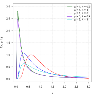
In probability theory, the inverse Gaussian distribution is a two-parameter family of continuous probability distributions with support on (0,∞).
In statistics, the multivariate t-distribution is a multivariate probability distribution. It is a generalization to random vectors of the Student's t-distribution, which is a distribution applicable to univariate random variables. While the case of a random matrix could be treated within this structure, the matrix t-distribution is distinct and makes particular use of the matrix structure.
A ratio distribution is a probability distribution constructed as the distribution of the ratio of random variables having two other known distributions. Given two random variables X and Y, the distribution of the random variable Z that is formed as the ratio Z = X/Y is a ratio distribution.

In probability theory and statistics, the half-normal distribution is a special case of the folded normal distribution.
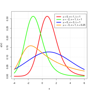
In probability theory, an exponentially modified Gaussian distribution describes the sum of independent normal and exponential random variables. An exGaussian random variable Z may be expressed as Z = X + Y, where X and Y are independent, X is Gaussian with mean μ and variance σ2, and Y is exponential of rate λ. It has a characteristic positive skew from the exponential component.
In statistics and probability theory, the nonparametric skew is a statistic occasionally used with random variables that take real values. It is a measure of the skewness of a random variable's distribution—that is, the distribution's tendency to "lean" to one side or the other of the mean. Its calculation does not require any knowledge of the form of the underlying distribution—hence the name nonparametric. It has some desirable properties: it is zero for any symmetric distribution; it is unaffected by a scale shift; and it reveals either left- or right-skewness equally well. In some statistical samples it has been shown to be less powerful than the usual measures of skewness in detecting departures of the population from normality.
In probability theory and statistics, cokurtosis is a measure of how much two random variables change together. Cokurtosis is the fourth standardized cross central moment. If two random variables exhibit a high level of cokurtosis they will tend to undergo extreme positive and negative deviations at the same time.


