First-hitting-time model

More colloquially, a first passage time in a stochastic system, is the time taken for a state variable to reach a certain value. Understanding this metric allows one to further understand the physical system under observation, and as such has been the topic of research in very diverse fields, from economics to ecology. ^[1]

The idea that a first hitting time of a stochastic process might describe the time to occurrence of an event has a long history, starting with an interest in the first passage time of Wiener diffusion processes in economics and then in physics in the early 1900s. ^{[2] [3] [4]} Modeling the probability of financial ruin as a first passage time was an early application in the field of insurance. ^[5] An interest in the mathematical properties of first-hitting-times and statistical models and methods for analysis of survival data appeared steadily between the middle and end of the 20th century. ^{[6] [7] [8] [9] [10]}

Examples

A common example of a first-hitting-time model is a ruin problem, such as Gambler's ruin. In this example, an entity (often described as a gambler or an insurance company) has an amount of money which varies randomly with time, possibly with some drift. The model considers the event that the amount of money reaches 0, representing bankruptcy. The model can answer questions such as the probability that this occurs within finite time, or the mean time until which it occurs.

First-hitting-time models can be applied to expected lifetimes, of patients or mechanical devices. When the process reaches an adverse threshold state for the first time, the patient dies, or the device breaks down.

A financial application of the first hitting time probability has been developed by Marcello Minenna in order to compute the minimum investment time horizon. ^{[11] [12]}

First passage time of a 1D Brownian particle

One of the simplest and omnipresent stochastic systems is that of the Brownian particle in one dimension. This system describes the motion of a particle which moves stochastically in one dimensional space, with equal probability of moving to the left or to the right. Given that Brownian motion is used often as a tool to understand more complex phenomena, it is important to understand the probability of a first passage time of the Brownian particle of reaching some position distant from its start location. This is done through the following means.

The probability density function (PDF) for a particle in one dimension is found by solving the one-dimensional diffusion equation. (This equation states that the position probability density diffuses outward over time. It is analogous to say, cream in a cup of coffee if the cream was all contained within some small location initially. After a long time the cream has diffused throughout the entire drink evenly.) Namely,

${\displaystyle {\frac {\partial p(x,t\mid x_{0})}{\partial t}}=D{\frac {\partial ^{2}p(x,t\mid x_{0})}{\partial x^{2}}},}$

given the initial condition ${\displaystyle p(x,t={0}\mid x_{0})=\delta (x-x_{0})}$; where ${\displaystyle x(t)}$ is the position of the particle at some given time, ${\displaystyle x_{0}}$ is the tagged particle's initial position, and ${\displaystyle D}$ is the diffusion constant with the S.I. units ${\displaystyle m^{2}s^{-1}}$ (an indirect measure of the particle's speed). The bar in the argument of the instantaneous probability refers to the conditional probability. The diffusion equation states that the rate of change over time in the probability of finding the particle at ${\displaystyle x(t)}$ position depends on the deceleration over distance of such probability at that position.

It can be shown that the one-dimensional PDF is

${\displaystyle p(x,t;x_{0})={\frac {1}{\sqrt {4\pi Dt}}}\exp \left(-{\frac {(x-x_{0})^{2}}{4Dt}}\right).}$

This states that the probability of finding the particle at ${\displaystyle x(t)}$ is Gaussian, and the width of the Gaussian is time dependent. More specifically the Full Width at Half Maximum (FWHM) – technically, this is actually the Full Duration at Half Maximum as the independent variable is time – scales like

${\displaystyle {\rm {FWHM}}\sim {\sqrt {t}}.}$

Using the PDF one is able to derive the average of a given function, ${\displaystyle L}$, at time ${\displaystyle t}$:

${\displaystyle \langle L(t)\rangle \equiv \int _{-\infty }^{\infty }L(x,t)p(x,t)\,dx,}$

where the average is taken over all space (or any applicable variable).

The First Passage Time Density (FPTD) is the probability that a particle has first reached a point ${\displaystyle x_{c}}$ at exactly time ${\displaystyle t}$ (not at some time during the interval up to ${\displaystyle t}$). This probability density is calculable from the Survival probability (a more common probability measure in statistics). Consider the absorbing boundary condition ${\displaystyle p(x_{c},t)=0}$ (The subscript c for the absorption point ${\displaystyle x_{c}}$ is an abbreviation for cliff used in many texts as an analogy to an absorption point). The PDF satisfying this boundary condition is given by

${\displaystyle p(x,t;x_{0},x_{c})={\frac {1}{\sqrt {4\pi Dt}}}\left(\exp \left(-{\frac {(x-x_{0})^{2}}{4Dt}}\right)-\exp \left(-{\frac {(x-(2x_{c}-x_{0}))^{2}}{4Dt}}\right)\right),}$

for ${\displaystyle x<x_{c}}$. The survival probability, the probability that the particle has remained at a position ${\displaystyle x<x_{c}}$ for all times up to ${\displaystyle t}$, is given by

${\displaystyle S(t)\equiv \int _{-\infty }^{x_{c}}p(x,t;x_{0},x_{c})\,dx=\operatorname {erf} \left({\frac {x_{c}-x_{0}}{2{\sqrt {Dt}}}}\right),}$

where ${\displaystyle \operatorname {erf} }$ is the error function. The relation between the Survival probability and the FPTD is as follows: the probability that a particle has reached the absorption point between times ${\displaystyle t}$ and ${\displaystyle t+dt}$ is ${\displaystyle f(t)\,dt=S(t)-S(t+dt)}$. If one uses the first-order Taylor approximation, the definition of the FPTD follows):

${\displaystyle f(t)=-{\frac {\partial S(t)}{\partial t}}.}$

By using the diffusion equation and integrating, the explicit FPTD is

${\displaystyle f(t)\equiv {\frac {|x_{c}-x_{0}|}{\sqrt {4\pi Dt^{3}}}}\exp \left(-{\frac {(x_{c}-x_{0})^{2}}{4Dt}}\right).}$

The first-passage time for a Brownian particle therefore follows a Lévy distribution.

For ${\displaystyle t\gg {\frac {(x_{c}-x_{0})^{2}}{4D}}}$, it follows from above that

${\displaystyle f(t)={\frac {\Delta x}{\sqrt {4\pi Dt^{3}}}}\sim t^{-3/2},}$

where ${\displaystyle \Delta x\equiv |x_{c}-x_{0}|}$. This equation states that the probability for a Brownian particle achieving a first passage at some long time (defined in the paragraph above) becomes increasingly small, but always finite.

The first moment of the FPTD diverges (as it is a so-called heavy-tailed distribution), therefore one cannot calculate the average FPT, so instead, one can calculate the typical time, the time when the FPTD is at a maximum (${\displaystyle \partial f/\partial t=0}$), i.e.,

${\displaystyle \tau _{\rm {ty}}={\frac {\Delta x^{2}}{6D}}.}$

First-hitting-time applications in many families of stochastic processes

First hitting times are central features of many families of stochastic processes, including Poisson processes, Wiener processes, gamma processes, and Markov chains, to name but a few. The state of the stochastic process may represent, for example, the strength of a physical system, the health of an individual, or the financial condition of a business firm. The system, individual or firm fails or experiences some other critical endpoint when the process reaches a threshold state for the first time. The critical event may be an adverse event (such as equipment failure, congested heart failure, or lung cancer) or a positive event (such as recovery from illness, discharge from hospital stay, child birth, or return to work after traumatic injury). The lapse of time until that critical event occurs is usually interpreted generically as a ‘survival time’. In some applications, the threshold is a set of multiple states so one considers competing first hitting times for reaching the first threshold in the set, as is the case when considering competing causes of failure in equipment or death for a patient.

Threshold regression: first-hitting-time regression

Practical applications of theoretical models for first hitting times often involve regression structures. When first hitting time models are equipped with regression structures, accommodating covariate data, we call such regression structure threshold regression. ^[13] The threshold state, parameters of the process, and even time scale may depend on corresponding covariates. Threshold regression as applied to time-to-event data has emerged since the start of this century and has grown rapidly, as described in a 2006 survey article ^[13] and its references. Connections between threshold regression models derived from first hitting times and the ubiquitous Cox proportional hazards regression model ^[14] was investigated in. ^[15] Applications of threshold regression range over many fields, including the physical and natural sciences, engineering, social sciences, economics and business, agriculture, health and medicine. ^{[16] [17] [18] [19] [20]}

Latent vs observable

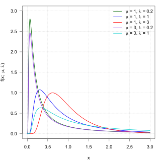
In many real world applications, a first-hitting-time (FHT) model has three underlying components: (1) a parent stochastic process${\displaystyle \{X(t)\}\,\,}$, which might be latent, (2) a threshold (or the barrier) and (3) a time scale. The first hitting time is defined as the time when the stochastic process first reaches the threshold. It is very important to distinguish whether the sample path of the parent process is latent (i.e., unobservable) or observable, and such distinction is a characteristic of the FHT model. By far, latent processes are most common. To give an example, we can use a Wiener process ${\displaystyle \{X(t),t\geq 0\,\}\,}$ as the parent stochastic process. Such Wiener process can be defined with the mean parameter ${\displaystyle {\mu }\,\,}$, the variance parameter ${\displaystyle {\sigma ^{2}}\,\,}$, and the initial value ${\displaystyle X(0)=x_{0}>0\,}$.

Operational or analytical time scale

The time scale of the stochastic process may be calendar or clock time or some more operational measure of time progression, such as mileage of a car, accumulated wear and tear on a machine component or accumulated exposure to toxic fumes. In many applications, the stochastic process describing the system state is latent or unobservable and its properties must be inferred indirectly from censored time-to-event data and/or readings taken over time on correlated processes, such as marker processes. The word ‘regression’ in threshold regression refers to first-hitting-time models in which one or more regression structures are inserted into the model in order to connect model parameters to explanatory variables or covariates. The parameters given regression structures may be parameters of the stochastic process, the threshold state and/or the time scale itself.

See also

• Survival analysis
• Proportional hazards models

References

1. Redner, S. (2001). A guide to first-passage processes. Cambridge university press.
2. Bachelier, L. Théorie de la spéculation. Annales scientifiques de l'École Normale Supérieure, Serie 3, Volume 17 (1900), pp. 21-86. doi : 10.24033/asens.476. http://www.numdam.org/articles/10.24033/asens.476/
3. Von E 1900
4. Smoluchowski 1915
5. Lundberg, F. (1903) Approximerad Framställning av Sannolikehetsfunktionen, Återförsäkering av Kollektivrisker, Almqvist & Wiksell, Uppsala.
6. Tweedie 1945
7. Tweedie 1957–1
8. Tweedie 1957–2
9. Whitmore 1970
10. Lancaster 1972
11. "Extended abstract".
12. "A Quantitative Framework to Assess the Risk-Reward Profile of non Equity Products".
13. Lee 2006
14. Cox 1972
15. Lee 2010
16. Aaron 2010
17. Chambaz 2014
18. Aaron 2015
19. He 2015
20. Hou 2016

• Whitmore, G. A. (1986). "First passage time models for duration data regression structures and competing risks". The Statistician. 35 (2): 207–219. doi:10.2307/2987525. JSTOR   2987525.
• Whitmore, G. A. (1995). "Estimating degradation by a Wiener diffusion process subject to measurement error". Lifetime Data Analysis. 1 (3): 307–319. doi:10.1007/BF00985762. PMID   9385107. S2CID   28077957.
• Whitmore, G. A.; Crowder, M. J.; Lawless, J. F. (1998). "Failure inference from a marker process based on a bivariate Wiener model". Lifetime Data Analysis. 4 (3): 229–251. doi:10.1023/A:1009617814586. PMID   9787604. S2CID   43301120.
• Redner, S. (2001). A Guide to First-Passage Processes. Cambridge University Press. ISBN   0-521-65248-0.
• Lee, M.-L. T.; Whitmore, G. A. (2006). "Threshold regression for survival analysis: Modeling event times by a stochastic process". Statistical Science. 21 (4): 501–513. arXiv: 0708.0346 . doi:10.1214/088342306000000330. S2CID   88518120.
• Bachelier, L. (1900). "Théorie de la Spéculation". Annales Scientifiques de l'École Normale Supérieure. 3 (17): 21–86. doi: 10.24033/asens.476 .
• Schrodinger, E. (1915). "Zur Theorie der Fall-und Steigversuche an Teilchen mit Brownscher Bewegung". Physikalische Zeitschrift. 16: 289–295.
• Smoluchowski, M. V. (1915). "Notiz über die Berechnung der Brownschen Molekularbewegung bei der Ehrenhaft-millikanschen Versuchsanordnung". Physikalische Zeitschrift. 16: 318–321.
• Lundberg, F. (1903). Approximerad Framställning av Sannolikehetsfunktionen, Återförsäkering av Kollektivrisker. Almqvist & Wiksell, Uppsala.
• Tweedie, M. C. K. (1945). "Inverse statistical variates". Nature. 155 (3937): 453. Bibcode:1945Natur.155..453T. doi: 10.1038/155453a0 .
• Tweedie, M. C. K. (1957). "Statistical properties of inverse Gaussian distributions – I". Annals of Mathematical Statistics. 28 (2): 362–377. doi: 10.1214/aoms/1177706964 .
• Tweedie, M. C. K. (1957). "Statistical properties of inverse Gaussian distributions – II". Annals of Mathematical Statistics. 28 (3): 696–705. doi: 10.1214/aoms/1177706881 .
• Whitmore, G. A.; Neufeldt, A. H. (1970). "An application of statistical models in mental health research". Bull. Math. Biophys. 32 (4): 563–579. doi:10.1007/BF02476771. PMID   5513393.
• Lancaster, T. (1972). "A stochastic model for the duration of a strike". J. Roy. Statist. Soc. Ser. A. 135 (2): 257–271. doi:10.2307/2344321. JSTOR   2344321.
• Cox, D. R. (1972). "Regression models and life tables (with discussion)". J R Stat Soc Ser B. 187: 187–230.
• Lee, M.-L. T.; Whitmore, G. A. (2010). "Threshold Proportional hazards and threshold regression: their theoretical and practical connections". Lifetime Data Analysis. 16 (2): 196–214. doi:10.1007/s10985-009-9138-0. PMC   6447409 . PMID   19960249.
• Aaron, S. D.; Ramsay, T.; Vandemheen, K.; Whitmore, G. A. (2010). "A threshold regression model for recurrent exacerbations in chronic obstructive pulmonary disease". Journal of Clinical Epidemiology. 63 (12): 1324–1331. doi:10.1016/j.jclinepi.2010.05.007. PMID   20800447.
• Chambaz, A.; Choudat, D.; Huber, C.; Pairon, J.; Van der Lann, M. J. (2014). "Analysis of occupational exposure to asbestos based on threshold regression modeling of case-control data". Biostatistics. 15 (2): 327–340. doi: 10.1093/biostatistics/kxt042 . PMID   24115271.
• Aaron, S. D.; Stephenson, A. L.; Cameron, D. W.; Whitmore, G. A. (2015). "A statistical model to predict one-year risk of death in patients with cystic fibrosis". Journal of Clinical Epidemiology. 68 (11): 1336–1345. doi:10.1016/j.jclinepi.2014.12.010. PMID   25655532.
• He, X.; Whitmore, G. A.; Loo, G. Y.; Hochberg, M. C.; Lee, M.-L. T. (2015). "A model for time to fracture with a shock stream superimposed on progressive degradation: the Study of Osteoporotic Fractures". Statistics in Medicine. 34 (4): 652–663. doi:10.1002/sim.6356. PMC   4314426 . PMID   25376757.
• Hou, W.-H.; Chuang, H.-Y.; Lee, M.-L. T. (2016). "A threshold regression model to predict return to work after traumatic limb injury". Injury. 47 (2): 483–489. doi:10.1016/j.injury.2015.11.032. PMID   26746983.