Wiener process

Wiener Process

Probability density function
Mean	${\displaystyle 0}$
Variance	${\displaystyle \sigma ^{2}t}$

A single realization of a one-dimensional Wiener process

A single realization of a three-dimensional Wiener process

In mathematics, the Wiener process is a real-valued continuous-time stochastic process named in honor of American mathematician Norbert Wiener for his investigations on the mathematical properties of the one-dimensional Brownian motion. ^[1] It is often also called Brownian motion due to its historical connection with the physical process of the same name originally observed by Scottish botanist Robert Brown. It is one of the best known Lévy processes (càdlàg stochastic processes with stationary independent increments) and occurs frequently in pure and applied mathematics, economics, quantitative finance, evolutionary biology, and physics.

The Wiener process plays an important role in both pure and applied mathematics. In pure mathematics, the Wiener process gave rise to the study of continuous time martingales. It is a key process in terms of which more complicated stochastic processes can be described. As such, it plays a vital role in stochastic calculus, diffusion processes and even potential theory. It is the driving process of Schramm–Loewner evolution. In applied mathematics, the Wiener process is used to represent the integral of a white noise Gaussian process, and so is useful as a model of noise in electronics engineering (see Brownian noise), instrument errors in filtering theory and disturbances in control theory.

The Wiener process has applications throughout the mathematical sciences. In physics it is used to study Brownian motion, the diffusion of minute particles suspended in fluid, and other types of diffusion via the Fokker–Planck and Langevin equations. It also forms the basis for the rigorous path integral formulation of quantum mechanics (by the Feynman–Kac formula, a solution to the Schrödinger equation can be represented in terms of the Wiener process) and the study of eternal inflation in physical cosmology. It is also prominent in the mathematical theory of finance, in particular the Black–Scholes option pricing model.

Characterisations of the Wiener process

The Wiener process ${\displaystyle W_{t}}$ is characterised by the following properties: ^[2]

1. ${\displaystyle W_{0}=0}$ almost surely
2. ${\displaystyle W}$ has independent increments: for every ${\displaystyle t>0,}$ the future increments ${\displaystyle W_{t+u}-W_{t},}$${\displaystyle u\geq 0,}$ are independent of the past values ${\displaystyle W_{s}}$, ${\displaystyle s<t.}$
3. ${\displaystyle W}$ has Gaussian increments: ${\displaystyle W_{t+u}-W_{t}}$ is normally distributed with mean ${\displaystyle 0}$ and variance ${\displaystyle u}$, ${\displaystyle W_{t+u}-W_{t}\sim {\mathcal {N}}(0,u).}$
4. ${\displaystyle W}$ has almost surely continuous paths: ${\displaystyle W_{t}}$ is almost surely continuous in ${\displaystyle t}$.

That the process has independent increments means that if 0 ≤ s₁ < t₁ ≤ s₂ < t₂ then W_t1 − W_s1 and W_t2 − W_s2 are independent random variables, and the similar condition holds for n increments.

An alternative characterisation of the Wiener process is the so-called Lévy characterisation that says that the Wiener process is an almost surely continuous martingale with W₀ = 0 and quadratic variation [W_t, W_t] = t (which means that W_t² − t is also a martingale).

A third characterisation is that the Wiener process has a spectral representation as a sine series whose coefficients are independent N(0, 1) random variables. This representation can be obtained using the Karhunen–Loève theorem.

Another characterisation of a Wiener process is the definite integral (from time zero to time t) of a zero mean, unit variance, delta correlated ("white") Gaussian process. ^[3]

The Wiener process can be constructed as the scaling limit of a random walk, or other discrete-time stochastic processes with stationary independent increments. This is known as Donsker's theorem. Like the random walk, the Wiener process is recurrent in one or two dimensions (meaning that it returns almost surely to any fixed neighborhood of the origin infinitely often) whereas it is not recurrent in dimensions three and higher (where a multidimensional Wiener process is a process such that its coordinates are independent Wiener processes). ^[4] Unlike the random walk, it is scale invariant, meaning that

$${\displaystyle \alpha ^{-1}W_{\alpha ^{2}t}}$$

is a Wiener process for any nonzero constant α. The Wiener measure is the probability law on the space of continuous functions g, with g(0) = 0, induced by the Wiener process. An integral based on Wiener measure may be called a Wiener integral.

Wiener process as a limit of random walk

Let ${\displaystyle \xi _{1},\xi _{2},\ldots }$ be i.i.d. random variables with mean 0 and variance 1. For each n, define a continuous time stochastic process

$${\displaystyle W_{n}(t)={\frac {1}{\sqrt {n}}}\sum \limits _{1\leq k\leq \lfloor nt\rfloor }\xi _{k},\qquad t\in [0,1].}$$

This is a random step function. Increments of ${\displaystyle W_{n}}$ are independent because the ${\displaystyle \xi _{k}}$ are independent. For large n, ${\displaystyle W_{n}(t)-W_{n}(s)}$ is close to ${\displaystyle N(0,t-s)}$ by the central limit theorem. Donsker's theorem asserts that as ${\displaystyle n\to \infty }$, ${\displaystyle W_{n}}$ approaches a Wiener process, which explains the ubiquity of Brownian motion. ^[5]

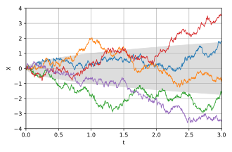
Properties of a one-dimensional Wiener process

Five sampled processes, with expected standard deviation in gray.

Basic properties

The unconditional probability density function follows a normal distribution with mean = 0 and variance = t, at a fixed time t:

$${\displaystyle f_{W_{t}}(x)={\frac {1}{\sqrt {2\pi t}}}e^{-x^{2}/(2t)}.}$$

The expectation is zero:

$${\displaystyle \operatorname {E} [W_{t}]=0.}$$

The variance, using the computational formula, is t:

$${\displaystyle \operatorname {Var} (W_{t})=t.}$$

These results follow immediately from the definition that increments have a normal distribution, centered at zero. Thus

$${\displaystyle W_{t}=W_{t}-W_{0}\sim N(0,t).}$$

Covariance and correlation

The covariance and correlation (where ${\displaystyle s\leq t}$):

$${\displaystyle {\begin{aligned}\operatorname {cov} (W_{s},W_{t})&=s,\\\operatorname {corr} (W_{s},W_{t})&={\frac {\operatorname {cov} (W_{s},W_{t})}{\sigma _{W_{s}}\sigma _{W_{t}}}}={\frac {s}{\sqrt {st}}}={\sqrt {\frac {s}{t}}}.\end{aligned}}}$$

These results follow from the definition that non-overlapping increments are independent, of which only the property that they are uncorrelated is used. Suppose that ${\displaystyle t_{1}\leq t_{2}}$.

$${\displaystyle \operatorname {cov} (W_{t_{1}},W_{t_{2}})=\operatorname {E} \left[(W_{t_{1}}-\operatorname {E} [W_{t_{1}}])\cdot (W_{t_{2}}-\operatorname {E} [W_{t_{2}}])\right]=\operatorname {E} \left[W_{t_{1}}\cdot W_{t_{2}}\right].}$$

Substituting

$${\displaystyle W_{t_{2}}=(W_{t_{2}}-W_{t_{1}})+W_{t_{1}}}$$

we arrive at:

$${\displaystyle {\begin{aligned}\operatorname {E} [W_{t_{1}}\cdot W_{t_{2}}]&=\operatorname {E} \left[W_{t_{1}}\cdot ((W_{t_{2}}-W_{t_{1}})+W_{t_{1}})\right]\\&=\operatorname {E} \left[W_{t_{1}}\cdot (W_{t_{2}}-W_{t_{1}})\right]+\operatorname {E} \left[W_{t_{1}}^{2}\right].\end{aligned}}}$$

Since ${\displaystyle W_{t_{1}}=W_{t_{1}}-W_{t_{0}}}$ and ${\displaystyle W_{t_{2}}-W_{t_{1}}}$ are independent,

$${\displaystyle \operatorname {E} \left[W_{t_{1}}\cdot (W_{t_{2}}-W_{t_{1}})\right]=\operatorname {E} [W_{t_{1}}]\cdot \operatorname {E} [W_{t_{2}}-W_{t_{1}}]=0.}$$

Thus

$${\displaystyle \operatorname {cov} (W_{t_{1}},W_{t_{2}})=\operatorname {E} \left[W_{t_{1}}^{2}\right]=t_{1}.}$$

A corollary useful for simulation is that we can write, for t₁ < t₂:

$${\displaystyle W_{t_{2}}=W_{t_{1}}+{\sqrt {t_{2}-t_{1}}}\cdot Z}$$

where Z is an independent standard normal variable.

Wiener representation

Wiener (1923) also gave a representation of a Brownian path in terms of a random Fourier series. If ${\displaystyle \xi _{n}}$ are independent Gaussian variables with mean zero and variance one, then

$${\displaystyle W_{t}=\xi _{0}t+{\sqrt {2}}\sum _{n=1}^{\infty }\xi _{n}{\frac {\sin \pi nt}{\pi n}}}$$

and

$${\displaystyle W_{t}={\sqrt {2}}\sum _{n=1}^{\infty }\xi _{n}{\frac {\sin \left(\left(n-{\frac {1}{2}}\right)\pi t\right)}{\left(n-{\frac {1}{2}}\right)\pi }}}$$

represent a Brownian motion on ${\displaystyle [0,1]}$. The scaled process

$${\displaystyle {\sqrt {c}}\,W\left({\frac {t}{c}}\right)}$$

is a Brownian motion on ${\displaystyle [0,c]}$ (cf. Karhunen–Loève theorem).

Running maximum

The joint distribution of the running maximum

$${\displaystyle M_{t}=\max _{0\leq s\leq t}W_{s}}$$

and W_t is

$${\displaystyle f_{M_{t},W_{t}}(m,w)={\frac {2(2m-w)}{t{\sqrt {2\pi t}}}}e^{-{\frac {(2m-w)^{2}}{2t}}},\qquad m\geq 0,w\leq m.}$$

To get the unconditional distribution of ${\displaystyle f_{M_{t}}}$, integrate over −∞ < w ≤ m:

$${\displaystyle {\begin{aligned}f_{M_{t}}(m)&=\int _{-\infty }^{m}f_{M_{t},W_{t}}(m,w)\,dw=\int _{-\infty }^{m}{\frac {2(2m-w)}{t{\sqrt {2\pi t}}}}e^{-{\frac {(2m-w)^{2}}{2t}}}\,dw\\[5pt]&={\sqrt {\frac {2}{\pi t}}}e^{-{\frac {m^{2}}{2t}}},\qquad m\geq 0,\end{aligned}}}$$

the probability density function of a Half-normal distribution. The expectation ^[6] is

$${\displaystyle \operatorname {E} [M_{t}]=\int _{0}^{\infty }mf_{M_{t}}(m)\,dm=\int _{0}^{\infty }m{\sqrt {\frac {2}{\pi t}}}e^{-{\frac {m^{2}}{2t}}}\,dm={\sqrt {\frac {2t}{\pi }}}}$$

If at time ${\displaystyle t}$ the Wiener process has a known value ${\displaystyle W_{t}}$, it is possible to calculate the conditional probability distribution of the maximum in interval ${\displaystyle [0,t]}$ (cf. Probability distribution of extreme points of a Wiener stochastic process). The cumulative probability distribution function of the maximum value, conditioned by the known value ${\displaystyle W_{t}}$, is:

$${\displaystyle \,F_{M_{W_{t}}}(m)=\Pr \left(M_{W_{t}}=\max _{0\leq s\leq t}W(s)\leq m\mid W(t)=W_{t}\right)=\ 1-\ e^{-2{\frac {m(m-W_{t})}{t}}}\ \,,\,\ \ m>\max(0,W_{t})}$$

Self-similarity

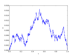
A demonstration of Brownian scaling, showing ${\displaystyle V_{t}=(1/{\sqrt {c}})W_{ct}}$ for decreasing c. Note that the average features of the function do not change while zooming in, and note that it zooms in quadratically faster horizontally than vertically.

Brownian scaling

For every c > 0 the process ${\displaystyle V_{t}=(1/{\sqrt {c}})W_{ct}}$ is another Wiener process.

Time reversal

The process ${\displaystyle V_{t}=W_{1}-W_{1-t}}$ for 0 ≤ t ≤ 1 is distributed like W_t for 0 ≤ t ≤ 1.

Time inversion

The process ${\displaystyle V_{t}=tW_{1/t}}$ is another Wiener process.

Projective invariance

Consider a Wiener process ${\displaystyle W(t)}$, ${\displaystyle t\in \mathbb {R} }$, conditioned so that ${\displaystyle \lim _{t\to \pm \infty }tW(t)=0}$ (which holds almost surely) and as usual ${\displaystyle W(0)=0}$. Then the following are all Wiener processes ( Takenaka 1988 ):

$${\displaystyle {\begin{array}{rcl}W_{1,s}(t)&=&W(t+s)-W(s),\quad s\in \mathbb {R} \\W_{2,\sigma }(t)&=&\sigma ^{-1/2}W(\sigma t),\quad \sigma >0\\W_{3}(t)&=&tW(-1/t).\end{array}}}$$

Thus the Wiener process is invariant under the projective group PSL(2,R), being invariant under the generators of the group. The action of an element ${\displaystyle g={\begin{bmatrix}a&b\\c&d\end{bmatrix}}}$ is ${\displaystyle W_{g}(t)=(ct+d)W\left({\frac {at+b}{ct+d}}\right)-ctW\left({\frac {a}{c}}\right)-dW\left({\frac {b}{d}}\right),}$ which defines a group action, in the sense that ${\displaystyle (W_{g})_{h}=W_{gh}.}$

Conformal invariance in two dimensions

Let ${\displaystyle W(t)}$ be a two-dimensional Wiener process, regarded as a complex-valued process with ${\displaystyle W(0)=0\in \mathbb {C} }$. Let ${\displaystyle D\subset \mathbb {C} }$ be an open set containing 0, and ${\displaystyle \tau _{D}}$ be associated Markov time:

$${\displaystyle \tau _{D}=\inf\{t\geq 0|W(t)\not \in D\}.}$$

If ${\displaystyle f:D\to \mathbb {C} }$ is a holomorphic function which is not constant, such that ${\displaystyle f(0)=0}$, then ${\displaystyle f(W_{t})}$ is a time-changed Wiener process in ${\displaystyle f(D)}$( Lawler 2005 ). More precisely, the process ${\displaystyle Y(t)}$ is Wiener in ${\displaystyle D}$ with the Markov time ${\displaystyle S(t)}$ where

$${\displaystyle Y(t)=f(W(\sigma (t)))}$$

$${\displaystyle S(t)=\int _{0}^{t}|f'(W(s))|^{2}\,ds}$$

$${\displaystyle \sigma (t)=S^{-1}(t):\quad t=\int _{0}^{\sigma (t)}|f'(W(s))|^{2}\,ds.}$$

A class of Brownian martingales

If a polynomial p(x, t) satisfies the partial differential equation

$${\displaystyle \left({\frac {\partial }{\partial t}}-{\frac {1}{2}}{\frac {\partial ^{2}}{\partial x^{2}}}\right)p(x,t)=0}$$

then the stochastic process

$${\displaystyle M_{t}=p(W_{t},t)}$$

is a martingale.

Example:${\displaystyle W_{t}^{2}-t}$ is a martingale, which shows that the quadratic variation of W on [0, t] is equal to t. It follows that the expected time of first exit of W from (−c, c) is equal to c².

More generally, for every polynomial p(x, t) the following stochastic process is a martingale:

$${\displaystyle M_{t}=p(W_{t},t)-\int _{0}^{t}a(W_{s},s)\,\mathrm {d} s,}$$

where a is the polynomial

$${\displaystyle a(x,t)=\left({\frac {\partial }{\partial t}}+{\frac {1}{2}}{\frac {\partial ^{2}}{\partial x^{2}}}\right)p(x,t).}$$

Example:${\displaystyle p(x,t)=\left(x^{2}-t\right)^{2},}$${\displaystyle a(x,t)=4x^{2};}$ the process

$${\displaystyle \left(W_{t}^{2}-t\right)^{2}-4\int _{0}^{t}W_{s}^{2}\,\mathrm {d} s}$$

is a martingale, which shows that the quadratic variation of the martingale ${\displaystyle W_{t}^{2}-t}$ on [0, t] is equal to

$${\displaystyle 4\int _{0}^{t}W_{s}^{2}\,\mathrm {d} s.}$$

About functions p(xa, t) more general than polynomials, see local martingales.

Some properties of sample paths

The set of all functions w with these properties is of full Wiener measure. That is, a path (sample function) of the Wiener process has all these properties almost surely.

Qualitative properties

• For every ε > 0, the function w takes both (strictly) positive and (strictly) negative values on (0, ε).
• The function w is continuous everywhere but differentiable nowhere (like the Weierstrass function).
• For any ${\displaystyle \epsilon >0}$, ${\displaystyle w(t)}$ is almost surely not ${\displaystyle ({\tfrac {1}{2}}+\epsilon )}$-Hölder continuous, and almost surely ${\displaystyle ({\tfrac {1}{2}}-\epsilon )}$-Hölder continuous. ^[7]
• Points of local maximum of the function w are a dense countable set; the maximum values are pairwise different; each local maximum is sharp in the following sense: if w has a local maximum at t then
  $${\displaystyle \lim _{s\to t}{\frac {|w(s)-w(t)|}{|s-t|}}\to \infty .}$$
  The same holds for local minima.
• The function w has no points of local increase, that is, no t > 0 satisfies the following for some ε in (0, t): first, w(s) ≤ w(t) for all s in (t − ε, t), and second, w(s) ≥ w(t) for all s in (t, t + ε). (Local increase is a weaker condition than that w is increasing on (t − ε, t + ε).) The same holds for local decrease.
• The function w is of unbounded variation on every interval.
• The quadratic variation of w over [0,t] is t.
• Zeros of the function w are a nowhere dense perfect set of Lebesgue measure 0 and Hausdorff dimension 1/2 (therefore, uncountable).

Quantitative properties

Law of the iterated logarithm

$${\displaystyle \limsup _{t\to +\infty }{\frac {|w(t)|}{\sqrt {2t\log \log t}}}=1,\quad {\text{almost surely}}.}$$

Modulus of continuity

Local modulus of continuity:

$${\displaystyle \limsup _{\varepsilon \to 0+}{\frac {|w(\varepsilon )|}{\sqrt {2\varepsilon \log \log(1/\varepsilon )}}}=1,\qquad {\text{almost surely}}.}$$

Global modulus of continuity (Lévy):

$${\displaystyle \limsup _{\varepsilon \to 0+}\sup _{0\leq s<t\leq 1,t-s\leq \varepsilon }{\frac {|w(s)-w(t)|}{\sqrt {2\varepsilon \log(1/\varepsilon )}}}=1,\qquad {\text{almost surely}}.}$$

Dimension doubling theorem

The dimension doubling theorems say that the Hausdorff dimension of a set under a Brownian motion doubles almost surely.

Local time

The image of the Lebesgue measure on [0, t] under the map w (the pushforward measure) has a density L_t. Thus,

$${\displaystyle \int _{0}^{t}f(w(s))\,\mathrm {d} s=\int _{-\infty }^{+\infty }f(x)L_{t}(x)\,\mathrm {d} x}$$

for a wide class of functions f (namely: all continuous functions; all locally integrable functions; all non-negative measurable functions). The density L_t is (more exactly, can and will be chosen to be) continuous. The number L_t(x) is called the local time at x of w on [0, t]. It is strictly positive for all x of the interval (a, b) where a and b are the least and the greatest value of w on [0, t], respectively. (For x outside this interval the local time evidently vanishes.) Treated as a function of two variables x and t, the local time is still continuous. Treated as a function of t (while x is fixed), the local time is a singular function corresponding to a nonatomic measure on the set of zeros of w.

These continuity properties are fairly non-trivial. Consider that the local time can also be defined (as the density of the pushforward measure) for a smooth function. Then, however, the density is discontinuous, unless the given function is monotone. In other words, there is a conflict between good behavior of a function and good behavior of its local time. In this sense, the continuity of the local time of the Wiener process is another manifestation of non-smoothness of the trajectory.

Information rate

The information rate of the Wiener process with respect to the squared error distance, i.e. its quadratic rate-distortion function, is given by ^[8]

$${\displaystyle R(D)={\frac {2}{\pi ^{2}\ln 2D}}\approx 0.29D^{-1}.}$$

Therefore, it is impossible to encode ${\displaystyle \{w_{t}\}_{t\in [0,T]}}$ using a binary code of less than ${\displaystyle TR(D)}$ bits and recover it with expected mean squared error less than ${\displaystyle D}$. On the other hand, for any ${\displaystyle \varepsilon >0}$, there exists ${\displaystyle T}$ large enough and a binary code of no more than ${\displaystyle 2^{TR(D)}}$ distinct elements such that the expected mean squared error in recovering ${\displaystyle \{w_{t}\}_{t\in [0,T]}}$ from this code is at most ${\displaystyle D-\varepsilon }$.

In many cases, it is impossible to encode the Wiener process without sampling it first. When the Wiener process is sampled at intervals ${\displaystyle T_{s}}$ before applying a binary code to represent these samples, the optimal trade-off between code rate ${\displaystyle R(T_{s},D)}$ and expected mean square error ${\displaystyle D}$ (in estimating the continuous-time Wiener process) follows the parametric representation ^[9]

$${\displaystyle R(T_{s},D_{\theta })={\frac {T_{s}}{2}}\int _{0}^{1}\log _{2}^{+}\left[{\frac {S(\varphi )-{\frac {1}{6}}}{\theta }}\right]d\varphi ,}$$

$${\displaystyle D_{\theta }={\frac {T_{s}}{6}}+T_{s}\int _{0}^{1}\min \left\{S(\varphi )-{\frac {1}{6}},\theta \right\}d\varphi ,}$$

where ${\displaystyle S(\varphi )=(2\sin(\pi \varphi /2))^{-2}}$ and ${\displaystyle \log ^{+}[x]=\max\{0,\log(x)\}}$. In particular, ${\displaystyle T_{s}/6}$ is the mean squared error associated only with the sampling operation (without encoding).

Related processes

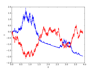
Wiener processes with drift (blue) and without drift (red).

2D Wiener processes with drift (blue) and without drift (red).

The generator of a Brownian motion is 1⁄2 times the Laplace–Beltrami operator. The image above is of the Brownian motion on a special manifold: the surface of a sphere.

The stochastic process defined by

$${\displaystyle X_{t}=\mu t+\sigma W_{t}}$$

is called a Wiener process with drift μ and infinitesimal variance σ². These processes exhaust continuous Lévy processes, which means that they are the only continuous Lévy processes, as a consequence of the Lévy–Khintchine representation.

Two random processes on the time interval [0, 1] appear, roughly speaking, when conditioning the Wiener process to vanish on both ends of [0,1]. With no further conditioning, the process takes both positive and negative values on [0, 1] and is called Brownian bridge. Conditioned also to stay positive on (0, 1), the process is called Brownian excursion. ^[10] In both cases a rigorous treatment involves a limiting procedure, since the formula P(A|B) = P(A ∩ B)/P(B) does not apply when P(B) = 0.

A geometric Brownian motion can be written

$${\displaystyle e^{\mu t-{\frac {\sigma ^{2}t}{2}}+\sigma W_{t}}.}$$

It is a stochastic process which is used to model processes that can never take on negative values, such as the value of stocks.

The stochastic process

$${\displaystyle X_{t}=e^{-t}W_{e^{2t}}}$$

is distributed like the Ornstein–Uhlenbeck process with parameters ${\displaystyle \theta =1}$, ${\displaystyle \mu =0}$, and ${\displaystyle \sigma ^{2}=2}$.

The time of hitting a single point x > 0 by the Wiener process is a random variable with the Lévy distribution. The family of these random variables (indexed by all positive numbers x) is a left-continuous modification of a Lévy process. The right-continuous modification of this process is given by times of first exit from closed intervals [0, x].

The local time L = (L^x_t)_{x ∈ R, t ≥ 0} of a Brownian motion describes the time that the process spends at the point x. Formally

$${\displaystyle L^{x}(t)=\int _{0}^{t}\delta (x-B_{t})\,ds}$$

where δ is the Dirac delta function. The behaviour of the local time is characterised by Ray–Knight theorems.

Brownian martingales

Let A be an event related to the Wiener process (more formally: a set, measurable with respect to the Wiener measure, in the space of functions), and X_t the conditional probability of A given the Wiener process on the time interval [0, t] (more formally: the Wiener measure of the set of trajectories whose concatenation with the given partial trajectory on [0, t] belongs to A). Then the process X_t is a continuous martingale. Its martingale property follows immediately from the definitions, but its continuity is a very special fact – a special case of a general theorem stating that all Brownian martingales are continuous. A Brownian martingale is, by definition, a martingale adapted to the Brownian filtration; and the Brownian filtration is, by definition, the filtration generated by the Wiener process.

Integrated Brownian motion

The time-integral of the Wiener process

$${\displaystyle W^{(-1)}(t):=\int _{0}^{t}W(s)\,ds}$$

is called integrated Brownian motion or integrated Wiener process. It arises in many applications and can be shown to have the distribution N(0, t³/3), ^[11] calculated using the fact that the covariance of the Wiener process is ${\displaystyle t\wedge s=\min(t,s)}$. ^[12]

For the general case of the process defined by

$${\displaystyle V_{f}(t)=\int _{0}^{t}f'(s)W(s)\,ds=\int _{0}^{t}(f(t)-f(s))\,dW_{s}}$$

Then, for ${\displaystyle a>0}$,

$${\displaystyle \operatorname {Var} (V_{f}(t))=\int _{0}^{t}(f(t)-f(s))^{2}\,ds}$$

$${\displaystyle \operatorname {cov} (V_{f}(t+a),V_{f}(t))=\int _{0}^{t}(f(t+a)-f(s))(f(t)-f(s))\,ds}$$

In fact, ${\displaystyle V_{f}(t)}$ is always a zero mean normal random variable. This allows for simulation of ${\displaystyle V_{f}(t+a)}$ given ${\displaystyle V_{f}(t)}$ by taking

$${\displaystyle V_{f}(t+a)=A\cdot V_{f}(t)+B\cdot Z}$$

where Z is a standard normal variable and

$${\displaystyle A={\frac {\operatorname {cov} (V_{f}(t+a),V_{f}(t))}{\operatorname {Var} (V_{f}(t))}}}$$

$${\displaystyle B^{2}=\operatorname {Var} (V_{f}(t+a))-A^{2}\operatorname {Var} (V_{f}(t))}$$

The case of ${\displaystyle V_{f}(t)=W^{(-1)}(t)}$ corresponds to ${\displaystyle f(t)=t}$. All these results can be seen as direct consequences of Itô isometry. The n-times-integrated Wiener process is a zero-mean normal variable with variance ${\displaystyle {\frac {t}{2n+1}}\left({\frac {t^{n}}{n!}}\right)^{2}}$. This is given by the Cauchy formula for repeated integration.

Time change

Every continuous martingale (starting at the origin) is a time changed Wiener process.

Example: 2W_t = V(4t) where V is another Wiener process (different from W but distributed like W).

Example.${\displaystyle W_{t}^{2}-t=V_{A(t)}}$ where ${\displaystyle A(t)=4\int _{0}^{t}W_{s}^{2}\,\mathrm {d} s}$ and V is another Wiener process.

In general, if M is a continuous martingale then ${\displaystyle M_{t}-M_{0}=V_{A(t)}}$ where A(t) is the quadratic variation of M on [0, t], and V is a Wiener process.

Corollary. (See also Doob's martingale convergence theorems) Let M_t be a continuous martingale, and

$${\displaystyle M_{\infty }^{-}=\liminf _{t\to \infty }M_{t},}$$

$${\displaystyle M_{\infty }^{+}=\limsup _{t\to \infty }M_{t}.}$$

Then only the following two cases are possible:

$${\displaystyle -\infty <M_{\infty }^{-}=M_{\infty }^{+}<+\infty ,}$$

$${\displaystyle -\infty =M_{\infty }^{-}<M_{\infty }^{+}=+\infty$$ ;}

other cases (such as ${\displaystyle M_{\infty }^{-}=M_{\infty }^{+}=+\infty ,}$ ${\displaystyle M_{\infty }^{-}<M_{\infty }^{+}<+\infty }$ etc.) are of probability 0.

Especially, a nonnegative continuous martingale has a finite limit (as t → ∞) almost surely.

All stated (in this subsection) for martingales holds also for local martingales.

Change of measure

A wide class of continuous semimartingales (especially, of diffusion processes) is related to the Wiener process via a combination of time change and change of measure.

Using this fact, the qualitative properties stated above for the Wiener process can be generalized to a wide class of continuous semimartingales. ^{[13] [14]}

Complex-valued Wiener process

The complex-valued Wiener process may be defined as a complex-valued random process of the form ${\displaystyle Z_{t}=X_{t}+iY_{t}}$ where ${\displaystyle X_{t}}$ and ${\displaystyle Y_{t}}$ are independent Wiener processes (real-valued). ^[15]

Self-similarity

Brownian scaling, time reversal, time inversion: the same as in the real-valued case.

Rotation invariance: for every complex number ${\displaystyle c}$ such that ${\displaystyle |c|=1}$ the process ${\displaystyle c\cdot Z_{t}}$ is another complex-valued Wiener process.

Time change

If ${\displaystyle f}$ is an entire function then the process ${\displaystyle f(Z_{t})-f(0)}$ is a time-changed complex-valued Wiener process.

Example:${\displaystyle Z_{t}^{2}=\left(X_{t}^{2}-Y_{t}^{2}\right)+2X_{t}Y_{t}i=U_{A(t)}}$ where

$${\displaystyle A(t)=4\int _{0}^{t}|Z_{s}|^{2}\,\mathrm {d} s}$$

and ${\displaystyle U}$ is another complex-valued Wiener process.

In contrast to the real-valued case, a complex-valued martingale is generally not a time-changed complex-valued Wiener process. For example, the martingale ${\displaystyle 2X_{t}+iY_{t}}$ is not (here ${\displaystyle X_{t}}$ and ${\displaystyle Y_{t}}$ are independent Wiener processes, as before).

Brownian sheet

Main article: Brownian sheet

The Brownian sheet is a multiparamateric generalization. The definition varies from authors, some define the Brownian sheet to have specifically a two-dimensional time parameter ${\displaystyle t}$ while others define it for general dimensions.

See also

Generalities: Abstract Wiener space Classical Wiener space Chernoff's distribution Fractal Brownian web Probability distribution of extreme points of a Wiener stochastic process

Numerical path sampling: Euler–Maruyama method Walk-on-spheres method

Notes

1. N.Wiener Collected Works vol.1
2. Durrett, Rick (2019). "Brownian Motion". Probability: Theory and Examples (5th ed.). Cambridge University Press. ISBN   9781108591034.
3. Huang, Steel T.; Cambanis, Stamatis (1978). "Stochastic and Multiple Wiener Integrals for Gaussian Processes". The Annals of Probability. 6 (4): 585–614. doi: 10.1214/aop/1176995480 . ISSN   0091-1798. JSTOR   2243125.
4. "Pólya's Random Walk Constants". Wolfram Mathworld.
5. Steven Lalley, Mathematical Finance 345 Lecture 5: Brownian Motion (2001)
6. Shreve, Steven E (2008). Stochastic Calculus for Finance II: Continuous Time Models. Springer. p. 114. ISBN   978-0-387-40101-0.
7. Mörters, Peter; Peres, Yuval; Schramm, Oded; Werner, Wendelin (2010). Brownian motion. Cambridge series in statistical and probabilistic mathematics. Cambridge: Cambridge University Press. p. 18. ISBN   978-0-521-76018-8.
8. T. Berger, "Information rates of Wiener processes," in IEEE Transactions on Information Theory, vol. 16, no. 2, pp. 134-139, March 1970. doi: 10.1109/TIT.1970.1054423
9. Kipnis, A., Goldsmith, A.J. and Eldar, Y.C., 2019. The distortion-rate function of sampled Wiener processes. IEEE Transactions on Information Theory, 65(1), pp.482-499.
10. Vervaat, W. (1979). "A relation between Brownian bridge and Brownian excursion". Annals of Probability . 7 (1): 143–149. doi: 10.1214/aop/1176995155 . JSTOR   2242845.
11. "Interview Questions VII: Integrated Brownian Motion – Quantopia". www.quantopia.net. Retrieved 2017-05-14.
12. Forum, "Variance of integrated Wiener process", 2009.
13. Revuz, D., & Yor, M. (1999). Continuous martingales and Brownian motion (Vol. 293). Springer.
14. Doob, J. L. (1953). Stochastic processes (Vol. 101). Wiley: New York.
15. Navarro-moreno, J.; Estudillo-martinez, M.D; Fernandez-alcala, R.M.; Ruiz-molina, J.C. (2009), "Estimation of Improper Complex-Valued Random Signals in Colored Noise by Using the Hilbert Space Theory", IEEE Transactions on Information Theory, 55 (6): 2859–2867, doi:10.1109/TIT.2009.2018329, S2CID   5911584

References

• Kleinert, Hagen (2004). Path Integrals in Quantum Mechanics, Statistics, Polymer Physics, and Financial Markets (4th ed.). Singapore: World Scientific. ISBN   981-238-107-4. (also available online: PDF-files)
• Lawler, Greg (2005), Conformally invariant processes in the plane, AMS.
• Stark, Henry; Woods, John (2002). Probability and Random Processes with Applications to Signal Processing (3rd ed.). New Jersey: Prentice Hall. ISBN   0-13-020071-9.
• Revuz, Daniel; Yor, Marc (1994). Continuous martingales and Brownian motion (Second ed.). Springer-Verlag.
• Takenaka, Shigeo (1988), "On pathwise projective invariance of Brownian motion", Proc Japan Acad, 64: 41–44.

External links

• Brownian Motion for the School-Going Child
• Brownian Motion, "Diverse and Undulating"
• Discusses history, botany and physics of Brown's original observations, with videos
• "Einstein's prediction finally witnessed one century later"  : a test to observe the velocity of Brownian motion
• "Interactive Web Application: Stochastic Processes used in Quantitative Finance".