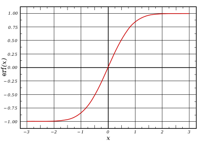
In statistics, for non-negative values of x, the error function has the following interpretation: for a random variableY that is normally distributed with mean 0 and standard deviation1/√2, erf x is the probability that Y falls in the range [−x, x].
Two closely related functions are the complementary error function (erfc) defined as
and the imaginary error function (erfi) defined as
The name "error function" and its abbreviation erf were proposed by J. W. L. Glaisher in 1871 on account of its connection with "the theory of Probability, and notably the theory of Errors."[3] The error function complement was also discussed by Glaisher in a separate publication in the same year.[4] For the "law of facility" of errors whose density is given by
(the normal distribution), Glaisher calculates the probability of an error lying between p and q as:
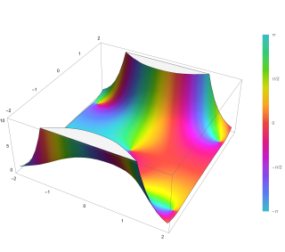
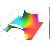
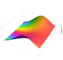
Plot of the error function Erf(z) in the complex plane from -2-2i to 2+2i with colors created with Mathematica 13.1 function ComplexPlot3D
Applications
When the results of a series of measurements are described by a normal distribution with standard deviationσ and expected value 0, then erf (a/σ√2) is the probability that the error of a single measurement lies between −a and +a, for positive a. This is useful, for example, in determining the bit error rate of a digital communication system.
The error function and its approximations can be used to estimate results that hold with high probability or with low probability. Given a random variable X ~ Norm[μ,σ] (a normal distribution with mean μ and standard deviation σ) and a constant L > μ, it can be shown via integration by substitution:
where A and B are certain numeric constants. If L is sufficiently far from the mean, specifically μ − L ≥ σ√ln k, then:
so the probability goes to 0 as k → ∞.
The probability for X being in the interval [La, Lb] can be derived as
Properties
Plots in the complex plane
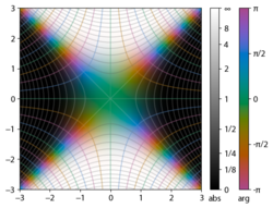
Integrand exp(−z2)
erf z
The property erf (−z) = −erf z means that the error function is an odd function. This directly results from the fact that the integrand e−t2 is an even function (the antiderivative of an even function which is zero at the origin is an odd function and vice versa).
The integrand f = exp(−z2) and f = erf z are shown in the complex z-plane in the figures at right with domain coloring.
The error function at +∞ is exactly 1 (see Gaussian integral). At the real axis, erf z approaches unity at z → +∞ and −1 at z → −∞. At the imaginary axis, it tends to ±i∞.
Taylor series
The error function is an entire function; it has no singularities (except that at infinity) and its Taylor expansion always converges, but is famously known "[...] for its bad convergence if x > 1."[5]
An expansion,[7] which converges more rapidly for all real values of x than a Taylor expansion, is obtained by using Hans Heinrich Bürmann's theorem:[8]
where sgn is the sign function. By keeping only the first two coefficients and choosing c1 = 31/200 and c2 = −341/8000, the resulting approximation shows its largest relative error at x = ±1.3796, where it is less than 0.0036127:
Inverse functions
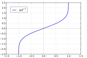
Inverse error function
Given a complex number z, there is not a unique complex number w satisfying erf w = z, so a true inverse function would be multivalued. However, for −1 < x < 1, there is a unique real number denoted erf−1x satisfying
The inverse error function is usually defined with domain (−1,1), and it is restricted to this domain in many computer algebra systems. However, it can be extended to the disk |z| < 1 of the complex plane, using the Maclaurin series[9]
where c0 = 1 and
So we have the series expansion (common factors have been canceled from numerators and denominators):
(After cancellation the numerator/denominator fractions are entries OEIS:A092676/OEIS:A092677 in the OEIS; without cancellation the numerator terms are given in entry OEIS:A002067.) The error function's value at±∞ is equal to±1.
For |z| < 1, we have erf(erf−1z) = z.
The inverse complementary error function is defined as
For real x, there is a unique real number erfi−1x satisfying erfi(erfi−1x) = x. The inverse imaginary error function is defined as erfi−1x.[10]
For any real x, Newton's method can be used to compute erfi−1x, and for −1 ≤ x ≤ 1, the following Maclaurin series converges:
where ck is defined as above.
Asymptotic expansion
A useful asymptotic expansion of the complementary error function (and therefore also of the error function) for large real x is
where (2n − 1)!! is the double factorial of (2n − 1), which is the product of all odd numbers up to (2n − 1). This series diverges for every finite x, and its meaning as asymptotic expansion is that for any integer N ≥ 1 one has
where the remainder is
which follows easily by induction, writing
and integrating by parts.
The asymptotic behavior of the remainder term, in Landau notation, is
as x → ∞. This can be found by
For large enough values of x, only the first few terms of this asymptotic expansion are needed to obtain a good approximation of erfc x (while for not too large values of x, the above Taylor expansion at 0 provides a very fast convergence).
Abramowitz and Stegun give several approximations of varying accuracy (equations 7.1.25–28). This allows one to choose the fastest approximation suitable for a given application. In order of increasing accuracy, they are:
where p = 0.3275911, a1 = 0.254829592, a2 = −0.284496736, a3 = 1.421413741, a4 = −1.453152027, a5 = 1.061405429
All of these approximations are valid for x ≥ 0. To use these approximations for negative x, use the fact that erf x is an odd function, so erf x = −erf(−x).
Exponential bounds and a pure exponential approximation for the complementary error function are given by[15]
The above have been generalized to sums of N exponentials[16] with increasing accuracy in terms of N so that erfc x can be accurately approximated or bounded by 2Q̃(√2x), where
In particular, there is a systematic methodology to solve the numerical coefficients {(an,bn)}N n = 1 that yield a minimax approximation or bound for the closely related Q-function: Q(x) ≈ Q̃(x), Q(x) ≤ Q̃(x), or Q(x) ≥ Q̃(x) for x ≥ 0. The coefficients {(an,bn)}N n = 1 for many variations of the exponential approximations and bounds up to N = 25 have been released to open access as a comprehensive dataset.[17]
A tight approximation of the complementary error function for x ∈ [0,∞) is given by Karagiannidis & Lioumpas (2007)[18] who showed for the appropriate choice of parameters {A,B} that
They determined {A,B} = {1.98,1.135}, which gave a good approximation for all x ≥ 0. Alternative coefficients are also available for tailoring accuracy for a specific application or transforming the expression into a tight bound.[19]
where the parameter β can be picked to minimize error on the desired interval of approximation.
Another approximation is given by Sergei Winitzki using his "global Padé approximations":[21][22]:2–3
where
This is designed to be very accurate in a neighborhood of 0 and a neighborhood of infinity, and the relative error is less than 0.00035 for all real x. Using the alternate value a ≈ 0.147 reduces the maximum relative error to about 0.00013.[23]
This approximation can be inverted to obtain an approximation for the inverse error function:
An approximation with a maximal error of 1.2×10⁻⁷ for any real argument is:[24]
with
and
An approximation of with a maximum relative error less than in absolute value is:[25] for ,
and for
A simple approximation for real-valued arguments could be done through Hyperbolic functions:
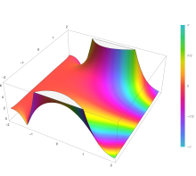
The complementary error function, denoted erfc, is defined as
Plot of the complementary error function Erfc(z) in the complex plane from -2-2i to 2+2i with colors created with Mathematica 13.1 function ComplexPlot3D
which also defines erfcx, the scaled complementary error function[26] (which can be used instead of erfc to avoid arithmetic underflow[26][27]). Another form of erfc x for x ≥ 0 is known as Craig's formula, after its discoverer:[28]
This expression is valid only for positive values of x, but it can be used in conjunction with erfc x = 2 − erfc(−x) to obtain erfc(x) for negative values. This form is advantageous in that the range of integration is fixed and finite. An extension of this expression for the erfc of the sum of two non-negative variables is as follows:[29]
Imaginary error function
The imaginary error function, denoted erfi, is defined as
Plot of the imaginary error function Erfi(z) in the complex plane from -2-2i to 2+2i with colors created with Mathematica 13.1 function ComplexPlot3D
Despite the name "imaginary error function", erfi x is real when x is real.
When the error function is evaluated for arbitrary complex arguments z, the resulting complex error function is usually discussed in scaled form as the Faddeeva function:
Cumulative distribution function
The error function is essentially identical to the standard normal cumulative distribution function, denoted Φ, also named norm(x) by some software languages[citation needed], as they differ only by scaling and translation. Indeed,
the normal cumulative distribution function plotted in the complex plane
or rearranged for erf and erfc:
Consequently, the error function is also closely related to the Q-function, which is the tail probability of the standard normal distribution. The Q-function can be expressed in terms of the error function as
Some authors discuss the more general functions:[citation needed]
Notable cases are:
E0(x) is a straight line through the origin: E0(x) = x/e√π
E2(x) is the error function, erf x.
After division by n!, all the En for odd n look similar (but not identical) to each other. Similarly, the En for even n look similar (but not identical) to each other after a simple division by n!. All generalised error functions for n > 0 look similar on the positive x side of the graph.
libcerf, numeric C library for complex error functions, provides the complex functions cerf, cerfc, cerfcx and the real functions erfi, erfcx with approximately 13–14 digits precision, based on the Faddeeva function as implemented in the MIT Faddeeva Package
The function for complex arguments can be computed numerically as follows:
In integral calculus, an elliptic integral is one of a number of related functions defined as the value of certain integrals, which were first studied by Giulio Fagnano and Leonhard Euler. Their name originates from their originally arising in connection with the problem of finding the arc length of an ellipse.
In probability theory and statistics, a normal distribution or Gaussian distribution is a type of continuous probability distribution for a real-valued random variable. The general form of its probability density function is
In mathematics, Stirling's approximation is an asymptotic approximation for factorials. It is a good approximation, leading to accurate results even for small values of . It is named after James Stirling, though a related but less precise result was first stated by Abraham de Moivre.
Integration is the basic operation in integral calculus. While differentiation has straightforward rules by which the derivative of a complicated function can be found by differentiating its simpler component functions, integration does not, so tables of known integrals are often useful. This page lists some of the most common antiderivatives.
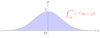
In mathematics, a Gaussian function, often simply referred to as a Gaussian, is a function of the base form
In probability theory and statistics, the Rayleigh distribution is a continuous probability distribution for nonnegative-valued random variables. Up to rescaling, it coincides with the chi distribution with two degrees of freedom. The distribution is named after Lord Rayleigh.
The Fresnel integralsS(x) and C(x) are two transcendental functions named after Augustin-Jean Fresnel that are used in optics and are closely related to the error function (erf). They arise in the description of near-field Fresnel diffraction phenomena and are defined through the following integral representations:
In mathematics, the inverse trigonometric functions are the inverse functions of the trigonometric functions. Specifically, they are the inverses of the sine, cosine, tangent, cotangent, secant, and cosecant functions, and are used to obtain an angle from any of the angle's trigonometric ratios. Inverse trigonometric functions are widely used in engineering, navigation, physics, and geometry.
In the physical sciences, the Airy function (or Airy function of the first kind) Ai(x) is a special function named after the British astronomer George Biddell Airy (1801–1892). The function Ai(x) and the related function Bi(x), are linearly independent solutions to the differential equation
In mathematics, the Clausen function, introduced by Thomas Clausen, is a transcendental, special function of a single variable. It can variously be expressed in the form of a definite integral, a trigonometric series, and various other forms. It is intimately connected with the polylogarithm, inverse tangent integral, polygamma function, Riemann zeta function, Dirichlet eta function, and Dirichlet beta function.
In mathematics, the Dawson function or Dawson integral (named after H. G. Dawson) is the one-sided Fourier–Laplace sine transform of the Gaussian function.
In mathematics, the Jacobi elliptic functions are a set of basic elliptic functions. They are found in the description of the motion of a pendulum, as well as in the design of electronic elliptic filters. While trigonometric functions are defined with reference to a circle, the Jacobi elliptic functions are a generalization which refer to other conic sections, the ellipse in particular. The relation to trigonometric functions is contained in the notation, for example, by the matching notation for . The Jacobi elliptic functions are used more often in practical problems than the Weierstrass elliptic functions as they do not require notions of complex analysis to be defined and/or understood. They were introduced by Carl Gustav Jakob Jacobi. Carl Friedrich Gauss had already studied special Jacobi elliptic functions in 1797, the lemniscate elliptic functions in particular, but his work was published much later.
The Gaussian integral, also known as the Euler–Poisson integral, is the integral of the Gaussian function over the entire real line. Named after the German mathematician Carl Friedrich Gauss, the integral is
In mathematical analysis, asymptotic analysis, also known as asymptotics, is a method of describing limiting behavior.
In mathematics, an asymptotic expansion, asymptotic series or Poincaré expansion is a formal series of functions which has the property that truncating the series after a finite number of terms provides an approximation to a given function as the argument of the function tends towards a particular, often infinite, point. Investigations by Dingle (1973) revealed that the divergent part of an asymptotic expansion is latently meaningful, i.e. contains information about the exact value of the expanded function.
The Voigt profile is a probability distribution given by a convolution of a Cauchy-Lorentz distribution and a Gaussian distribution. It is often used in analyzing data from spectroscopy or diffraction.
In mathematics, the lemniscate constantϖ is a transcendental mathematical constant that is the ratio of the perimeter of Bernoulli's lemniscate to its diameter, analogous to the definition of π for the circle. Equivalently, the perimeter of the lemniscate is 2ϖ. The lemniscate constant is closely related to the lemniscate elliptic functions and approximately equal to 2.62205755. The symbol ϖ is a cursive variant of π; see Pi § Variant pi.
In mathematics, the lemniscate elliptic functions are elliptic functions related to the arc length of the lemniscate of Bernoulli. They were first studied by Giulio Fagnano in 1718 and later by Leonhard Euler and Carl Friedrich Gauss, among others.
In statistics, the Q-function is the tail distribution function of the standard normal distribution. In other words, is the probability that a normal (Gaussian) random variable will obtain a value larger than standard deviations. Equivalently, is the probability that a standard normal random variable takes a value larger than .
↑ Dominici, Diego (2006). "Asymptotic analysis of the derivatives of the inverse error function". arXiv:math/0607230.
↑ Bergsma, Wicher (2006). "On a new correlation coefficient, its orthogonal decomposition and associated tests of independence". arXiv:math/0604627.
↑ Cuyt, Annie A. M.; Petersen, Vigdis B.; Verdonk, Brigitte; Waadeland, Haakon; Jones, William B. (2008). Handbook of Continued Fractions for Special Functions. Springer-Verlag. ISBN978-1-4020-6948-2.
↑ Ng, Edward W.; Geller, Murray (January 1969). "A table of integrals of the Error functions". Journal of Research of the National Bureau of Standards Section B. 73B (1): 1. doi:10.6028/jres.073B.001.
↑ Tanash, I.M.; Riihonen, T. (2020). "Global minimax approximations and bounds for the Gaussian Q-function by sums of exponentials". IEEE Transactions on Communications. 68 (10): 6514–6524. arXiv:2007.06939. doi:10.1109/TCOMM.2020.3006902. S2CID220514754.
↑ Tanash, I.M.; Riihonen, T. (2021). "Improved coefficients for the Karagiannidis–Lioumpas approximations and bounds to the Gaussian Q-function". IEEE Communications Letters. 25 (5): 1468–1471. arXiv:2101.07631. doi:10.1109/LCOMM.2021.3052257. S2CID231639206.
↑ Zeng, Caibin; Chen, Yang Cuan (2015). "Global Padé approximations of the generalized Mittag-Leffler function and its inverse". Fractional Calculus and Applied Analysis. 18 (6): 1492–1506. arXiv:1310.5592. doi:10.1515/fca-2015-0086. S2CID118148950. Indeed, Winitzki [32] provided the so-called global Padé approximation
↑ Behnad, Aydin (2020). "A Novel Extension to Craig's Q-Function Formula and Its Application in Dual-Branch EGC Performance Analysis". IEEE Transactions on Communications. 68 (7): 4117–4125. doi:10.1109/TCOMM.2020.2986209. S2CID216500014.
This page is based on this Wikipedia article Text is available under the CC BY-SA 4.0 license; additional terms may apply. Images, videos and audio are available under their respective licenses.


![Graph of generalised error functions En(x):
grey curve: E1(x) =
1 - e/[?]p
red curve: E2(x) = erf(x)
green curve: E3(x)
blue curve: E4(x)
gold curve: E5(x). Error Function Generalised.svg](http://upload.wikimedia.org/wikipedia/commons/thumb/0/02/Error_Function_Generalised.svg/400px-Error_Function_Generalised.svg.png)