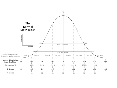
Standard score

"Standardize" redirects here. For industrial and technical standards, see Standardization.

"Z-score" redirects here. For other uses, see Z-score (disambiguation).

Comparison of the various grading methods in a normal distribution, including: standard deviations, cumulative percentages, percentile equivalents, z-scores, T-scores

In statistics, the standard score is the number of standard deviations by which the value of a raw score (i.e., an observed value or data point) is above or below the mean value of what is being observed or measured. Raw scores above the mean have positive standard scores, while those below the mean have negative standard scores.

It is calculated by subtracting the population mean from an individual raw score and then dividing the difference by the population standard deviation. This process of converting a raw score into a standard score is called standardizing or normalizing (however, "normalizing" can refer to many types of ratios; see Normalization for more).

Standard scores are most commonly called z-scores; the two terms may be used interchangeably, as they are in this article. Other equivalent terms in use include z-value, z-statistic, normal score, standardized variable and pull in high energy physics. ^{[1] [2]}

Computing a z-score requires knowledge of the mean and standard deviation of the complete population to which a data point belongs; if one only has a sample of observations from the population, then the analogous computation using the sample mean and sample standard deviation yields the t-statistic.

Calculation

If the population mean and population standard deviation are known, a raw score x is converted into a standard score by ^[3]

${\displaystyle z={x-\mu \over \sigma }}$

where:

μ is the mean of the population,

σ is the standard deviation of the population.

The absolute value of z represents the distance between that raw score x and the population mean in units of the standard deviation. z is negative when the raw score is below the mean, positive when above.

Calculating z using this formula requires use of the population mean and the population standard deviation, not the sample mean or sample deviation. However, knowing the true mean and standard deviation of a population is often an unrealistic expectation, except in cases such as standardized testing, where the entire population is measured.

When the population mean and the population standard deviation are unknown, the standard score may be estimated by using the sample mean and sample standard deviation as estimates of the population values. ^{[4] [5] [6] [7]}

In these cases, the z-score is given by

${\displaystyle z={x-{\bar {x}} \over S}}$

where:

${\displaystyle {\bar {x}}}$ is the mean of the sample,

S is the standard deviation of the sample.

Though it should always be stated, the distinction between use of the population and sample statistics often is not made. In either case, the numerator and denominator of the equations have the same units of measure so that the units cancel out through division and z is left as a dimensionless quantity.

Applications

Z-test

Main article: Z-test

The z-score is often used in the z-test in standardized testing – the analog of the Student's t-test for a population whose parameters are known, rather than estimated. As it is very unusual to know the entire population, the t-test is much more widely used.

Prediction intervals

The standard score can be used in the calculation of prediction intervals. A prediction interval [L,U], consisting of a lower endpoint designated L and an upper endpoint designated U, is an interval such that a future observation X will lie in the interval with high probability ${\displaystyle \gamma }$, i.e.

${\displaystyle P(L<X<U)=\gamma ,}$

For the standard score Z of X it gives: ^[8]

${\displaystyle P\left({\frac {L-\mu }{\sigma }}<Z<{\frac {U-\mu }{\sigma }}\right)=\gamma .}$

By determining the quantile z such that

${\displaystyle P\left(-z<Z<z\right)=\gamma }$

it follows:

${\displaystyle L=\mu -z\sigma ,\ U=\mu +z\sigma }$

Process control

In process control applications, the Z value provides an assessment of the degree to which a process is operating off-target.

Comparison of scores measured on different scales: ACT and SAT

The z score for Student A was 1, meaning Student A was 1 standard deviation above the mean. Thus, Student A performed in the 84.13 percentile on the SAT.

When scores are measured on different scales, they may be converted to z-scores to aid comparison. Dietz et al. ^[9] give the following example, comparing student scores on the (old) SAT and ACT high school tests. The table shows the mean and standard deviation for total scores on the SAT and ACT. Suppose that student A scored 1800 on the SAT, and student B scored 24 on the ACT. Which student performed better relative to other test-takers?

	SAT	ACT
Mean	1500	21
Standard deviation	300	5

The z score for Student B was 0.6, meaning Student B was 0.6 standard deviation above the mean. Thus, Student B performed in the 72.57 percentile on the SAT.

The z-score for student A is ${\displaystyle z={x-\mu \over \sigma }={1800-1500 \over 300}=1}$

The z-score for student B is ${\displaystyle z={x-\mu \over \sigma }={24-21 \over 5}=0.6}$

Because student A has a higher z-score than student B, student A performed better compared to other test-takers than did student B.

Percentage of observations below a z-score

Continuing the example of ACT and SAT scores, if it can be further assumed that both ACT and SAT scores are normally distributed (which is approximately correct), then the z-scores may be used to calculate the percentage of test-takers who received lower scores than students A and B.

Cluster analysis and multidimensional scaling

"For some multivariate techniques such as multidimensional scaling and cluster analysis, the concept of distance between the units in the data is often of considerable interest and importance… When the variables in a multivariate data set are on different scales, it makes more sense to calculate the distances after some form of standardization." ^[10]

Principal components analysis

In principal components analysis, "Variables measured on different scales or on a common scale with widely differing ranges are often standardized." ^[11]

Relative importance of variables in multiple regression: standardized regression coefficients

Standardization of variables prior to multiple regression analysis is sometimes used as an aid to interpretation. ^[12] (page 95) state the following.

"The standardized regression slope is the slope in the regression equation if X and Y are standardized … Standardization of X and Y is done by subtracting the respective means from each set of observations and dividing by the respective standard deviations … In multiple regression, where several X variables are used, the standardized regression coefficients quantify the relative contribution of each X variable."

However, Kutner et al. ^[13] (p 278) give the following caveat: "… one must be cautious about interpreting any regression coefficients, whether standardized or not. The reason is that when the predictor variables are correlated among themselves, … the regression coefficients are affected by the other predictor variables in the model … The magnitudes of the standardized regression coefficients are affected not only by the presence of correlations among the predictor variables but also by the spacings of the observations on each of these variables. Sometimes these spacings may be quite arbitrary. Hence, it is ordinarily not wise to interpret the magnitudes of standardized regression coefficients as reflecting the comparative importance of the predictor variables."

Standardizing in mathematical statistics

Further information: Normalization (statistics)

In mathematical statistics, a random variable X is standardized by subtracting its expected value ${\displaystyle \operatorname {E} [X]}$ and dividing the difference by its standard deviation ${\displaystyle \sigma (X)={\sqrt {\operatorname {Var} (X)}}:}$

${\displaystyle Z={X-\operatorname {E} [X] \over \sigma (X)}}$

If the random variable under consideration is the sample mean of a random sample ${\displaystyle \ X_{1},\dots ,X_{n}}$ of X:

${\displaystyle {\bar {X}}={1 \over n}\sum _{i=1}^{n}X_{i}}$

then the standardized version is

${\displaystyle Z={\frac {{\bar {X}}-\operatorname {E} [{\bar {X}}]}{\sigma (X)/{\sqrt {n}}}}}$

Where the standardised sample mean's variance was calculated as follows:

${\displaystyle {\begin{array}{l}\operatorname {Var} \left(\sum x_{i}\right)=\sum \operatorname {Var} (x_{i})=n\operatorname {Var} (x_{i})=n\sigma ^{2}\\\operatorname {Var} ({\overline {X}})=\operatorname {Var} \left({\frac {\sum x_{i}}{n}}\right)={\frac {1}{n^{2}}}\operatorname {Var} \left(\sum x_{i}\right)={\frac {n\sigma ^{2}}{n^{2}}}={\frac {\sigma ^{2}}{n}}\end{array}}}$

T-score

"T-score" redirects here. Not to be confused with t-statistic.

In educational assessment, T-score is a standard score Z shifted and scaled to have a mean of 50 and a standard deviation of 10. ^{[14] [15] [16]} It is also known as hensachi in Japanese, where the concept is much more widely known and used in the context of high school and university admissions.

In bone density measurements, the T-score is the standard score of the measurement compared to the population of healthy 30-year-old adults, and has the usual mean of 0 and standard deviation of 1. ^[17]

See also

• Normalization (statistics)
• Omega ratio
• Standard normal deviate
• Mahalanobis distance
• Error function
• Studentized residual

References

1. Mulders, Martijn; Zanderighi, Giulia, eds. (2017). 2015 European School of High-Energy Physics: Bansko, Bulgaria 02 - 15 Sep 2015. CERN Yellow Reports: School Proceedings. Geneva: CERN. ISBN   978-92-9083-472-4.
2. Gross, Eilam (2017-11-06). "Practical Statistics for High Energy Physics". CERN Yellow Reports: School Proceedings. 4/2017: 165–186. doi:10.23730/CYRSP-2017-004.165.
3. E. Kreyszig (1979). Advanced Engineering Mathematics (Fourth ed.). Wiley. p. 880, eq. 5. ISBN   0-471-02140-7.
4. Spiegel, Murray R.; Stephens, Larry J (2008), Schaum's Outlines Statistics (Fourth ed.), McGraw Hill, ISBN   978-0-07-148584-5
5. Mendenhall, William; Sincich, Terry (2007), Statistics for Engineering and the Sciences (Fifth ed.), Pearson / Prentice Hall, ISBN   978-0131877061
6. Glantz, Stanton A.; Slinker, Bryan K.; Neilands, Torsten B. (2016), Primer of Applied Regression & Analysis of Variance (Third ed.), McGraw Hill, ISBN   978-0071824118
7. Aho, Ken A. (2014), Foundational and Applied Statistics for Biologists (First ed.), Chapman & Hall / CRC Press, ISBN   978-1439873380
8. E. Kreyszig (1979). Advanced Engineering Mathematics (Fourth ed.). Wiley. p. 880, eq. 6. ISBN   0-471-02140-7.
9. Diez, David; Barr, Christopher; Çetinkaya-Rundel, Mine (2012), OpenIntro Statistics (Second ed.), openintro.org
10. Everitt, Brian; Hothorn, Torsten J (2011), An Introduction to Applied Multivariate Analysis with R, Springer, ISBN   978-1441996497
11. Johnson, Richard; Wichern, Wichern (2007), Applied Multivariate Statistical Analysis, Pearson / Prentice Hall
12. Afifi, Abdelmonem; May, Susanne K.; Clark, Virginia A. (2012), Practical Multivariate Analysis (Fifth ed.), Chapman & Hall/CRC, ISBN   978-1439816806
13. Kutner, Michael; Nachtsheim, Christopher; Neter, John (204), Applied Linear Regression Models (Fourth ed.), McGraw Hill, ISBN   978-0073014661
14. John Salvia; James Ysseldyke; Sara Witmer (29 January 2009). Assessment: In Special and Inclusive Education. Cengage Learning. pp. 43–. ISBN   978-0-547-13437-6.
15. Edward S. Neukrug; R. Charles Fawcett (1 January 2014). Essentials of Testing and Assessment: A Practical Guide for Counselors, Social Workers, and Psychologists. Cengage Learning. pp. 133–. ISBN   978-1-305-16183-2.
16. Randy W. Kamphaus (16 August 2005). Clinical Assessment of Child and Adolescent Intelligence. Springer. pp. 123–. ISBN   978-0-387-26299-4.
17. "Bone Mass Measurement: What the Numbers Mean". NIH Osteoporosis and Related Bone Diseases National Resource Center. National Institute of Health. Retrieved 5 August 2017.

Further reading

• Carroll, Susan Rovezzi; Carroll, David J. (2002). Statistics Made Simple for School Leaders (illustrated ed.). Rowman & Littlefield. ISBN   978-0-8108-4322-6 . Retrieved 7 June 2009.
• Larsen, Richard J.; Marx, Morris L. (2000). An Introduction to Mathematical Statistics and Its Applications (Third ed.). p. 282. ISBN   0-13-922303-7.

External links

• z-score calculator