T-statistic

Last updated

In statistics, the t-statistic is the ratio of the departure of the estimated value of a parameter from its hypothesized value to its standard error. It is used in hypothesis testing via Student's t-test. The t-statistic is used in a t-test to determine whether to support or reject the null hypothesis. It is very similar to the z-score but with the difference that t-statistic is used when the sample size is small or the population standard deviation is unknown. For example, the t-statistic is used in estimating the population mean from a sampling distribution of sample means if the population standard deviation is unknown. It is also used along with p-value when running hypothesis tests where the p-value tells us what the odds are of the results to have happened.

Contents

Definition and features

Let be an estimator of parameter β in some statistical model. Then a t-statistic for this parameter is any quantity of the form

where β0 is a non-random, known constant, which may or may not match the actual unknown parameter value β, and is the standard error of the estimator for β.

By default, statistical packages report t-statistic with β0 = 0 (these t-statistics are used to test the significance of corresponding regressor). However, when t-statistic is needed to test the hypothesis of the form H0: β = β0, then a non-zero β0 may be used.

If is an ordinary least squares estimator in the classical linear regression model (that is, with normally distributed and homoscedastic error terms), and if the true value of the parameter β is equal to β0, then the sampling distribution of the t-statistic is the Student's t-distribution with (nk) degrees of freedom, where n is the number of observations, and k is the number of regressors (including the intercept)[ citation needed ].

In the majority of models, the estimator is consistent for β and is distributed asymptotically normally. If the true value of the parameter β is equal to β0, and the quantity correctly estimates the asymptotic variance of this estimator, then the t-statistic will asymptotically have the standard normal distribution.

In some models the distribution of the t-statistic is different from the normal distribution, even asymptotically. For example, when a time series with a unit root is regressed in the augmented Dickey–Fuller test, the test t-statistic will asymptotically have one of the Dickey–Fuller distributions (depending on the test setting).

Use

Most frequently, t statistics are used in Student's t-tests, a form of statistical hypothesis testing, and in the computation of certain confidence intervals.

The key property of the t statistic is that it is a pivotal quantity – while defined in terms of the sample mean, its sampling distribution does not depend on the population parameters, and thus it can be used regardless of what these may be.

One can also divide a residual by the sample standard deviation:

to compute an estimate for the number of standard deviations a given sample is from the mean, as a sample version of a z-score, the z-score requiring the population parameters.

Prediction

Given a normal distribution with unknown mean and variance, the t-statistic of a future observation after one has made n observations, is an ancillary statistic – a pivotal quantity (does not depend on the values of μ and σ2) that is a statistic (computed from observations). This allows one to compute a frequentist prediction interval (a predictive confidence interval), via the following t-distribution:

Solving for yields the prediction distribution

from which one may compute predictive confidence intervals – given a probability p, one may compute intervals such that 100p% of the time, the next observation will fall in that interval.

History

The term "t-statistic" is abbreviated from "hypothesis test statistic". [1] [ citation needed ] In statistics, the t-distribution was first derived as a posterior distribution in 1876 by Helmert [2] [3] [4] and Lüroth. [5] [6] [7] The t-distribution also appeared in a more general form as Pearson Type IV distribution in Karl Pearson's 1895 paper. [8] However, the T-Distribution, also known as Student's T Distribution gets its name from William Sealy Gosset who was first to publish the result in English in his 1908 paper titled "The Probable Error of a Mean" (in Biometrika) using his pseudonym "Student" [9] [10] because his employer preferred their staff to use pen names when publishing scientific papers instead of their real name, so he used the name "Student" to hide his identity. [11] Gosset worked at the Guinness Brewery in Dublin, Ireland, and was interested in the problems of small samples – for example, the chemical properties of barley where sample sizes might be as few as 3. Hence a second version of the etymology of the term Student is that Guinness did not want their competitors to know that they were using the t-test to determine the quality of raw material. Although it was William Gosset after whom the term "Student" is penned, it was actually through the work of Ronald Fisher that the distribution became well known as "Student's distribution" [12] [13] and "Student's t-test"

See also

Related Research Articles

The likelihood function is the joint probability of observed data viewed as a function of the parameters of a statistical model.

<span class="mw-page-title-main">Least squares</span> Approximation method in statistics

The method of least squares is a standard approach in regression analysis to approximate the solution of overdetermined systems by minimizing the sum of the squares of the residuals made in the results of each individual equation.

Students <i>t</i>-distribution Probability distribution

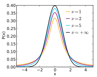
In probability and statistics, Student's t-distribution is a continuous probability distribution that generalizes the standard normal distribution. Like the latter, it is symmetric around zero and bell-shaped.

In statistical inference, specifically predictive inference, a prediction interval is an estimate of an interval in which a future observation will fall, with a certain probability, given what has already been observed. Prediction intervals are often used in regression analysis.

A t-test is a type of statistical analysis used to compare the averages of two groups and determine whether the differences between them are more likely to arise from random chance. It is any statistical hypothesis test in which the test statistic follows a Student's t-distribution under the null hypothesis. It is most commonly applied when the test statistic would follow a normal distribution if the value of a scaling term in the test statistic were known. When the scaling term is estimated based on the data, the test statistic—under certain conditions—follows a Student's t distribution. The t-test's most common application is to test whether the means of two populations are different.

<span class="mw-page-title-main">Regression analysis</span> Set of statistical processes for estimating the relationships among variables

In statistical modeling, regression analysis is a set of statistical processes for estimating the relationships between a dependent variable and one or more independent variables. The most common form of regression analysis is linear regression, in which one finds the line that most closely fits the data according to a specific mathematical criterion. For example, the method of ordinary least squares computes the unique line that minimizes the sum of squared differences between the true data and that line. For specific mathematical reasons, this allows the researcher to estimate the conditional expectation of the dependent variable when the independent variables take on a given set of values. Less common forms of regression use slightly different procedures to estimate alternative location parameters or estimate the conditional expectation across a broader collection of non-linear models.

<span class="mw-page-title-main">Nonlinear regression</span> Regression analysis

In statistics, nonlinear regression is a form of regression analysis in which observational data are modeled by a function which is a nonlinear combination of the model parameters and depends on one or more independent variables. The data are fitted by a method of successive approximations.

<span class="mw-page-title-main">Consistent estimator</span> Statistical estimator converging in probability to a true parameter as sample size increases

In statistics, a consistent estimator or asymptotically consistent estimator is an estimator—a rule for computing estimates of a parameter θ0—having the property that as the number of data points used increases indefinitely, the resulting sequence of estimates converges in probability to θ0. This means that the distributions of the estimates become more and more concentrated near the true value of the parameter being estimated, so that the probability of the estimator being arbitrarily close to θ0 converges to one.

In statistics, the Wald test assesses constraints on statistical parameters based on the weighted distance between the unrestricted estimate and its hypothesized value under the null hypothesis, where the weight is the precision of the estimate. Intuitively, the larger this weighted distance, the less likely it is that the constraint is true. While the finite sample distributions of Wald tests are generally unknown, it has an asymptotic χ2-distribution under the null hypothesis, a fact that can be used to determine statistical significance.

In statistics, a probit model is a type of regression where the dependent variable can take only two values, for example married or not married. The word is a portmanteau, coming from probability + unit. The purpose of the model is to estimate the probability that an observation with particular characteristics will fall into a specific one of the categories; moreover, classifying observations based on their predicted probabilities is a type of binary classification model.

In statistics, ordinary least squares (OLS) is a type of linear least squares method for choosing the unknown parameters in a linear regression model by the principle of least squares: minimizing the sum of the squares of the differences between the observed dependent variable in the input dataset and the output of the (linear) function of the independent variable.

In econometrics and statistics, the generalized method of moments (GMM) is a generic method for estimating parameters in statistical models. Usually it is applied in the context of semiparametric models, where the parameter of interest is finite-dimensional, whereas the full shape of the data's distribution function may not be known, and therefore maximum likelihood estimation is not applicable.

Weighted least squares (WLS), also known as weighted linear regression, is a generalization of ordinary least squares and linear regression in which knowledge of the unequal variance of observations (heteroscedasticity) is incorporated into the regression. WLS is also a specialization of generalized least squares, when all the off-diagonal entries of the covariance matrix of the errors, are null.

<span class="mw-page-title-main">Simple linear regression</span> Linear regression model with a single explanatory variable

In statistics, simple linear regression is a linear regression model with a single explanatory variable. That is, it concerns two-dimensional sample points with one independent variable and one dependent variable and finds a linear function that, as accurately as possible, predicts the dependent variable values as a function of the independent variable. The adjective simple refers to the fact that the outcome variable is related to a single predictor.

In statistics, M-estimators are a broad class of extremum estimators for which the objective function is a sample average. Both non-linear least squares and maximum likelihood estimation are special cases of M-estimators. The definition of M-estimators was motivated by robust statistics, which contributed new types of M-estimators. However, M-estimators are not inherently robust, as is clear from the fact that they include maximum likelihood estimators, which are in general not robust. The statistical procedure of evaluating an M-estimator on a data set is called M-estimation.

In statistics, the Durbin–Watson statistic is a test statistic used to detect the presence of autocorrelation at lag 1 in the residuals from a regression analysis. It is named after James Durbin and Geoffrey Watson. The small sample distribution of this ratio was derived by John von Neumann. Durbin and Watson applied this statistic to the residuals from least squares regressions, and developed bounds tests for the null hypothesis that the errors are serially uncorrelated against the alternative that they follow a first order autoregressive process. Note that the distribution of this test statistic does not depend on the estimated regression coefficients and the variance of the errors.

Bootstrapping is any test or metric that uses random sampling with replacement, and falls under the broader class of resampling methods. Bootstrapping assigns measures of accuracy to sample estimates. This technique allows estimation of the sampling distribution of almost any statistic using random sampling methods.

The topic of heteroskedasticity-consistent (HC) standard errors arises in statistics and econometrics in the context of linear regression and time series analysis. These are also known as heteroskedasticity-robust standard errors, Eicker–Huber–White standard errors, to recognize the contributions of Friedhelm Eicker, Peter J. Huber, and Halbert White.

In statistics, the Breusch–Godfrey test is used to assess the validity of some of the modelling assumptions inherent in applying regression-like models to observed data series. In particular, it tests for the presence of serial correlation that has not been included in a proposed model structure and which, if present, would mean that incorrect conclusions would be drawn from other tests or that sub-optimal estimates of model parameters would be obtained.

Denote a binary response index model as: , where .

References

  1. The Microbiome in Health and Disease. Academic Press. 29 May 2020. p. 397. ISBN   978-0-12-820001-8.
  2. Szabó, István (2003), "Systeme aus einer endlichen Anzahl starrer Körper", Einführung in die Technische Mechanik, Springer Berlin Heidelberg, pp. 196–199, doi:10.1007/978-3-642-61925-0_16, ISBN   978-3-540-13293-6
  3. Schlyvitch, B. (October 1937). "Untersuchungen über den anastomotischen Kanal zwischen der Arteria coeliaca und mesenterica superior und damit in Zusammenhang stehende Fragen". Zeitschrift für Anatomie und Entwicklungsgeschichte. 107 (6): 709–737. doi:10.1007/bf02118337. ISSN   0340-2061. S2CID   27311567.
  4. Helmert (1876). "Die Genauigkeit der Formel von Peters zur Berechnung des wahrscheinlichen Beobachtungsfehlers directer Beobachtungen gleicher Genauigkeit". Astronomische Nachrichten (in German). 88 (8–9): 113–131. Bibcode:1876AN.....88..113H. doi:10.1002/asna.18760880802.
  5. Lüroth, J. (1876). "Vergleichung von zwei Werthen des wahrscheinlichen Fehlers". Astronomische Nachrichten (in German). 87 (14): 209–220. Bibcode:1876AN.....87..209L. doi:10.1002/asna.18760871402.
  6. Pfanzagl, J. (1996). "Studies in the history of probability and statistics XLIV. A forerunner of the t-distribution". Biometrika . 83 (4): 891–898. doi:10.1093/biomet/83.4.891. MR   1766040.
  7. Sheynin, Oscar (1995). "Helmert's work in the theory of errors". Archive for History of Exact Sciences. 49 (1): 73–104. doi:10.1007/BF00374700. ISSN   0003-9519. S2CID   121241599.
  8. Pearson, Karl (1895). "X. Contributions to the mathematical theory of evolution.—II. Skew variation in homogeneous material". Philosophical Transactions of the Royal Society of London A. 186: 343–414. Bibcode:1895RSPTA.186..343P. doi: 10.1098/rsta.1895.0010 . ISSN   1364-503X.
  9. "Student" (William Sealy Gosset) (1908). "The Probable Error of a Mean". Biometrika . 6 (1): 1–25. doi:10.1093/biomet/6.1.1. hdl:10338.dmlcz/143545. JSTOR   2331554.
  10. "T Table | History of T Table, Etymology, one-tail T Table, two-tail T Table and T-statistic".
  11. Wendl, M. C. (2016). "Pseudonymous fame". Science. 351 (6280): 1406. doi:10.1126/science.351.6280.1406. PMID   27013722.
  12. Tuttle, Md; Anazonwu, Bs, Walter; Rubin, Md, Lee (2014). "Subgroup Analysis of Topical Tranexamic Acid in Total Knee Arthroplasty". Reconstructive Review. 4 (2): 37–41. doi: 10.15438/rr.v4i2.72 .
  13. Walpole, Ronald E. (2006). Probability & statistics for engineers & scientists. Myers, H. Raymond. (7th ed.). New Delhi: Pearson. ISBN   81-7758-404-9. OCLC   818811849.