Prediction interval

Not to be confused with Prediction error.

In statistical inference, specifically predictive inference, a prediction interval is an estimate of an interval in which a future observation will fall, with a certain probability, given what has already been observed. Prediction intervals are often used in regression analysis.

A simple example is given by a six-sided die with face values ranging from 1 to 6. The confidence interval for the estimated expected value of the face value will be around 3.5 and will become narrower with a larger sample size. However, the prediction interval for the next roll will approximately range from 1 to 6, even with any number of samples seen so far.

Prediction intervals are used in both frequentist statistics and Bayesian statistics: a prediction interval bears the same relationship to a future observation that a frequentist confidence interval or Bayesian credible interval bears to an unobservable population parameter: prediction intervals predict the distribution of individual future points, whereas confidence intervals and credible intervals of parameters predict the distribution of estimates of the true population mean or other quantity of interest that cannot be observed.

Introduction

If one makes the parametric assumption that the underlying distribution is a normal distribution, and has a sample set {X₁, ..., X_n}, then confidence intervals and credible intervals may be used to estimate the population mean μ and population standard deviation σ of the underlying population, while prediction intervals may be used to estimate the value of the next sample variable, X_n+1.

Alternatively, in Bayesian terms, a prediction interval can be described as a credible interval for the variable itself, rather than for a parameter of the distribution thereof.

The concept of prediction intervals need not be restricted to inference about a single future sample value but can be extended to more complicated cases. For example, in the context of river flooding where analyses are often based on annual values of the largest flow within the year, there may be interest in making inferences about the largest flood likely to be experienced within the next 50 years.

Since prediction intervals are only concerned with past and future observations, rather than unobservable population parameters, they are advocated as a better method than confidence intervals by some statisticians, such as Seymour Geisser,^{[ citation needed ]} following the focus on observables by Bruno de Finetti.^{[ citation needed ]}

Normal distribution

Given a sample from a normal distribution, whose parameters are unknown, it is possible to give prediction intervals in the frequentist sense, i.e., an interval [a, b] based on statistics of the sample such that on repeated experiments, X_n+1 falls in the interval the desired percentage of the time; one may call these "predictive confidence intervals". ^[1]

A general technique of frequentist prediction intervals is to find and compute a pivotal quantity of the observables X₁, ..., X_n, X_n+1 – meaning a function of observables and parameters whose probability distribution does not depend on the parameters – that can be inverted to give a probability of the future observation X_n+1 falling in some interval computed in terms of the observed values so far, ${\displaystyle X_{1},\dots ,X_{n}.}$ Such a pivotal quantity, depending only on observables, is called an ancillary statistic. ^[2] The usual method of constructing pivotal quantities is to take the difference of two variables that depend on location, so that location cancels out, and then take the ratio of two variables that depend on scale, so that scale cancels out. The most familiar pivotal quantity is the Student's t-statistic, which can be derived by this method and is used in the sequel.

Known mean, known variance

See also: 68–95–99.7 rule

A prediction interval [ℓ,u] for a future observation X in a normal distribution N(μ,σ²) with known mean and variance may be calculated from

${\displaystyle \gamma =P(\ell <X<u)=P\left({\frac {\ell -\mu }{\sigma }}<{\frac {X-\mu }{\sigma }}<{\frac {u-\mu }{\sigma }}\right)=P\left({\frac {\ell -\mu }{\sigma }}<Z<{\frac {u-\mu }{\sigma }}\right),}$

where ${\displaystyle Z={\frac {X-\mu }{\sigma }}}$, the standard score of X, is distributed as standard normal.

Hence

${\displaystyle {\frac {\ell -\mu }{\sigma }}=-z,\quad {\frac {u-\mu }{\sigma }}=z,}$

or

${\displaystyle \ell =\mu -z\sigma ,\quad u=\mu +z\sigma ,}$

with z the quantile in the standard normal distribution for which:

${\displaystyle \gamma =P(-z<Z<z).}$

or equivalently;

${\displaystyle {\tfrac {1}{2}}(1-\gamma )=P(Z>z).}$

Prediction interval	z
75%	1.15 [3]
90%	1.64 [3]
95%	1.96 [3]
99%	2.58 [3]

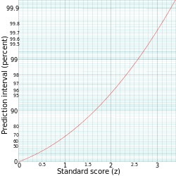
Prediction interval (on the y-axis) given from z (the quantile of the standard score, on the x-axis). The y-axis is logarithmically compressed (but the values on it are not modified).

The prediction interval is conventionally written as:

${\displaystyle \left[\mu -z\sigma ,\ \mu +z\sigma \right].}$

For example, to calculate the 95% prediction interval for a normal distribution with a mean (μ) of 5 and a standard deviation (σ) of 1, then z is approximately 2. Therefore, the lower limit of the prediction interval is approximately 5 ‒ (2⋅1) = 3, and the upper limit is approximately 5 + (2⋅1) = 7, thus giving a prediction interval of approximately 3 to 7.

Diagram showing the cumulative distribution function for the normal distribution with mean (μ) 0 and variance (σ ) 1. In addition to the quantile function, the prediction interval for any standard score can be calculated by (1 − (1 − Φ_μ,σ(standard score))⋅2). For example, a standard score of x = 1.96 gives Φ_μ,σ(1.96) = 0.9750 corresponding to a prediction interval of (1 − (1 − 0.9750)⋅2) = 0.9500 = 95%.

Estimation of parameters

For a distribution with unknown parameters, a direct approach to prediction is to estimate the parameters and then use the associated quantile function – for example, one could use the sample mean ${\displaystyle {\overline {X}}}$ as estimate for μ and the sample variance s² as an estimate for σ². There are two natural choices for s² here – dividing by ${\displaystyle (n-1)}$ yields an unbiased estimate, while dividing by n yields the maximum likelihood estimator, and either might be used. One then uses the quantile function with these estimated parameters ${\displaystyle \Phi _{{\overline {X}},s^{2}}^{-1}}$ to give a prediction interval.

This approach is usable, but the resulting interval will not have the repeated sampling interpretation ^[4] – it is not a predictive confidence interval.

For the sequel, use the sample mean:

${\displaystyle {\overline {X}}=(X_{1}+\cdots +X_{n})/n}$

and the (unbiased) sample variance:

${\displaystyle s^{2}={1 \over n-1}\sum _{i=1}^{n}(X_{i}-{\overline {X}})^{2}}$

Unknown mean, known variance

Given ^[5] a normal distribution with unknown mean μ but known variance ${\displaystyle \sigma ^{2}}$, the sample mean ${\displaystyle {\overline {X}}}$ of the observations ${\displaystyle X_{1},\dots ,X_{n}}$ has distribution ${\displaystyle N(\mu ,\sigma ^{2}/n),}$ while the future observation ${\displaystyle X_{n+1}}$ has distribution ${\displaystyle N(\mu ,\sigma ^{2}).}$ Taking the difference of these cancels the μ and yields a normal distribution of variance ${\displaystyle \sigma ^{2}+(\sigma ^{2}/n),}$ thus

${\displaystyle {\frac {X_{n+1}-{\overline {X}}}{\sqrt {\sigma ^{2}+(\sigma ^{2}/n)}}}\sim N(0,1).}$

Solving for ${\displaystyle X_{n+1}}$ gives the prediction distribution ${\displaystyle N({\overline {X}},\sigma ^{2}+(\sigma ^{2}/n)),}$ from which one can compute intervals as before. This is a predictive confidence interval in the sense that if one uses a quantile range of 100p%, then on repeated applications of this computation, the future observation ${\displaystyle X_{n+1}}$ will fall in the predicted interval 100p% of the time.

Notice that this prediction distribution is more conservative than using the estimated mean ${\displaystyle {\overline {X}}}$ and known variance ${\displaystyle \sigma ^{2}}$, as this uses compound variance ${\displaystyle \sigma ^{2}+(\sigma ^{2}/n)}$, hence yields slightly wider intervals. This is necessary for the desired confidence interval property to hold.

Known mean, unknown variance

Conversely, given a normal distribution with known mean μ but unknown variance ${\displaystyle \sigma ^{2}}$, the sample variance ${\displaystyle s^{2}}$ of the observations ${\displaystyle X_{1},\dots ,X_{n}}$ has, up to scale, a ${\displaystyle \chi _{n-1}^{2}}$ distribution; more precisely:

${\displaystyle {\frac {(n-1)s^{2}}{\sigma ^{2}}}\sim \chi _{n-1}^{2}.}$

On the other hand, the future observation ${\displaystyle X_{n+1}}$ has distribution ${\displaystyle N(\mu ,\sigma ^{2}).}$ Taking the ratio of the future observation residual ${\displaystyle X_{n+1}-\mu }$ and the sample standard deviation s cancels the σ, yielding a Student's t-distribution with n – 1 degrees of freedom (see its derivation):

${\displaystyle {\frac {X_{n+1}-\mu }{s}}\sim T^{n-1}.}$

Solving for ${\displaystyle X_{n+1}}$ gives the prediction distribution ${\displaystyle \mu \pm sT^{n-1},}$ from which one can compute intervals as before.

Notice that this prediction distribution is more conservative than using a normal distribution with the estimated standard deviation ${\displaystyle s}$ and known mean μ, as it uses the t-distribution instead of the normal distribution, hence yields wider intervals. This is necessary for the desired confidence interval property to hold.

Unknown mean, unknown variance

Combining the above for a normal distribution ${\displaystyle N(\mu ,\sigma ^{2})}$ with both μ and σ² unknown yields the following ancillary statistic: ^[6]

${\displaystyle {\frac {X_{n+1}-{\overline {X}}}{s{\sqrt {1+1/n}}}}\sim T^{n-1}}$

This simple combination is possible because the sample mean and sample variance of the normal distribution are independent statistics; this is only true for the normal distribution, and in fact characterizes the normal distribution.

Solving for ${\displaystyle X_{n+1}}$ yields the prediction distribution

${\displaystyle {\overline {X}}+s{\sqrt {1+1/n}}\cdot T^{n-1}}$

The probability of ${\displaystyle X_{n+1}}$ falling in a given interval is then:

${\displaystyle \Pr \left({\overline {X}}-T_{a}s{\sqrt {1+(1/n)}}\leq X_{n+1}\leq {\overline {X}}+T_{a}s{\sqrt {1+(1/n)}}\,\right)=p}$

where T_a is the 100((1 − p)/2)^th percentile of Student's t-distribution with n − 1 degrees of freedom. Therefore, the numbers

${\displaystyle {\overline {X}}\pm T_{a}s{\sqrt {1+(1/n)}}}$

are the endpoints of a 100(1 − p)% prediction interval for ${\displaystyle X_{n+1}}$.

Non-parametric methods

One can compute prediction intervals without any assumptions on the population, i.e. in a non-parametric way.

The residual bootstrap method can be used for constructing non-parametric prediction intervals.

Conformal Prediction

Main article: conformal prediction

In general the conformal prediction method is more general. Let us look at the special case of using the minimum and maximum as boundaries for a prediction interval: If one has a sample of identical random variables {X₁, ..., X_n}, then the probability that the next observation X_n+1 will be the largest is 1/(n + 1), since all observations have equal probability of being the maximum. In the same way, the probability that X_n+1 will be the smallest is 1/(n + 1). The other (n − 1)/(n + 1) of the time, X_n+1 falls between the sample maximum and sample minimum of the sample {X₁, ..., X_n}. Thus, denoting the sample maximum and minimum by M and m, this yields an (n − 1)/(n + 1) prediction interval of [m, M].

Notice that while this gives the probability that a future observation will fall in a range, it does not give any estimate as to where in a segment it will fall – notably, if it falls outside the range of observed values, it may be far outside the range. See extreme value theory for further discussion. Formally, this applies not just to sampling from a population, but to any exchangeable sequence of random variables, not necessarily independent or identically distributed.

Contrast with other intervals

Main article: Interval estimation

See also: Tolerance interval and Quantile regression

Contrast with confidence intervals

Main article: Confidence interval

In the formula for the predictive confidence interval no mention is made of the unobservable parameters μ and σ of population mean and standard deviation – the observed sample statistics ${\displaystyle {\overline {X}}_{n}}$ and ${\displaystyle S_{n}}$ of sample mean and standard deviation are used, and what is estimated is the outcome of future samples.

When considering prediction intervals, rather than using sample statistics as estimators of population parameters and applying confidence intervals to these estimates, one considers "the next sample" ${\displaystyle X_{n+1}}$ as itself a statistic, and computes its sampling distribution.

In parameter confidence intervals, one estimates population parameters; if one wishes to interpret this as prediction of the next sample, one models "the next sample" as a draw from this estimated population, using the (estimated) population distribution. By contrast, in predictive confidence intervals, one uses the sampling distribution of (a statistic of) a sample of n or n + 1 observations from such a population, and the population distribution is not directly used, though the assumption about its form (though not the values of its parameters) is used in computing the sampling distribution.

In regression analysis

Further information: Regression analysis § Prediction (interpolation and extrapolation), and Mean and predicted outcome

A common application of prediction intervals is to regression analysis. Suppose the data is being modeled by a straight line (simple linear regression):

${\displaystyle y_{i}=\alpha +\beta x_{i}+\varepsilon _{i}\,}$

where ${\displaystyle y_{i}}$ is the response variable, ${\displaystyle x_{i}}$ is the explanatory variable, ε_i is a random error term, and ${\displaystyle \alpha }$ and ${\displaystyle \beta }$ are parameters.

Given estimates ${\displaystyle {\hat {\alpha }}}$ and ${\displaystyle {\hat {\beta }}}$ for the parameters, such as from a ordinary least squares, the predicted response value y_d for a given explanatory value x_d is

${\displaystyle {\hat {y}}_{d}={\hat {\alpha }}+{\hat {\beta }}x_{d},}$

(the point on the regression line), while the actual response would be

${\displaystyle y_{d}=\alpha +\beta x_{d}+\varepsilon _{d}.\,}$

The point estimate ${\displaystyle {\hat {y}}_{d}}$ is called the mean response , and is an estimate of the expected value of y_d, ${\displaystyle E(y\mid x_{d}).}$

A prediction interval instead gives an interval in which one expects y_d to fall; this is not necessary if the actual parameters α and β are known (together with the error term ε_i), but if one is estimating from a sample, then one may use the standard error of the estimates for the intercept and slope (${\displaystyle {\hat {\alpha }}}$ and ${\displaystyle {\hat {\beta }}}$), as well as their correlation, to compute a prediction interval.

In regression, Faraway (2002 , p. 39) makes a distinction between intervals for predictions of the mean response vs. for predictions of observed response—affecting essentially the inclusion or not of the unity term within the square root in the expansion factors above; for details, see Faraway (2002).

Bayesian statistics

See also: Posterior predictive distribution

Seymour Geisser, a proponent of predictive inference, gives predictive applications of Bayesian statistics. ^[7]

In Bayesian statistics, one can compute (Bayesian) prediction intervals from the posterior probability of the random variable, as a credible interval. In theoretical work, credible intervals are not often calculated for the prediction of future events, but for inference of parameters – i.e., credible intervals of a parameter, not for the outcomes of the variable itself. However, particularly where applications are concerned with possible extreme values of yet to be observed cases, credible intervals for such values can be of practical importance.

Applications

Prediction intervals are commonly used as definitions of reference ranges, such as reference ranges for blood tests to give an idea of whether a blood test is normal or not. For this purpose, the most commonly used prediction interval is the 95% prediction interval, and a reference range based on it can be called a standard reference range.

See also

• Extrapolation
• Posterior probability
• Prediction
• Prediction band
• Seymour Geisser
• Statistical model validation
• Trend estimation

Notes

1. Geisser (1993 , p.  6 ): Chapter 2: Non-Bayesian predictive approaches
2. Geisser (1993 , p.  7 )
3. Table A2 in Sterne & Kirkwood (2003 , p. 472)
4. Geisser (1993 , pp.  8–9 )
5. Geisser (1993 , p.  7– )
6. Geisser (1993 , Example 2.2, p. 9–10 )
7. Geisser (1993)

References

• Faraway, Julian J. (2002), Practical Regression and Anova using R (PDF)
• Geisser, Seymour (1993), Predictive Inference, CRC Press
• Sterne, Jonathan; Kirkwood, Betty R. (2003), Essential Medical Statistics , Blackwell Science, ISBN   0-86542-871-9

Further reading

• Chatfield, C. (1993). "Calculating Interval Forecasts". Journal of Business & Economic Statistics . 11 (2): 121–135. doi:10.2307/1391361. JSTOR   1391361.
• Lawless, J. F.; Fredette, M. (2005). "Frequentist prediction intervals and predictive distributions". Biometrika . 92 (3): 529–542. doi: 10.1093/biomet/92.3.529 .
• Meade, N.; Islam, T. (1995). "Prediction Intervals for Growth Curve Forecasts". Journal of Forecasting . 14 (5): 413–430. doi:10.1002/for.3980140502.
• ISO 16269-8 Standard Interpretation of Data, Part 8, Determination of Prediction Intervals