Posterior predictive distribution

Last updated February 25, 2024

In Bayesian statistics, the posterior predictive distribution is the distribution of possible unobserved values conditional on the observed values.^[1]^[2]

It may seem tempting to plug in a single best estimate ${\hat {\theta }}$ for $\theta$ , but this ignores uncertainty about $\theta$ , and because a source of uncertainty is ignored, the predictive distribution will be too narrow. Put another way, predictions of extreme values of ${\tilde {x}}$ will have a lower probability than if the uncertainty in the parameters as given by their posterior distribution is accounted for.

A posterior predictive distribution accounts for uncertainty about $\theta$ . The posterior distribution of possible $\theta$ values depends on $\mathbf {X}$ :

p(\theta |\mathbf {X} )

And the posterior predictive distribution of ${\tilde {x}}$ given $\mathbf {X}$ is calculated by marginalizing the distribution of ${\tilde {x}}$ given $\theta$ over the posterior distribution of $\theta$ given $\mathbf {X}$ :

p({\tilde {x}}|\mathbf {X} )=\int _{\Theta }p({\tilde {x}}|\theta )\,p(\theta |\mathbf {X} )\operatorname {d} \!\theta

Because it accounts for uncertainty about $\theta$ , the posterior predictive distribution will in general be wider than a predictive distribution which plugs in a single best estimate for $\theta$ .

Prior vs. posterior predictive distribution

The prior predictive distribution, in a Bayesian context, is the distribution of a data point marginalized over its prior distribution $G$ . That is, if ${\tilde {x}}\sim F({\tilde {x}}|\theta )$ and $\theta \sim G(\theta |\alpha )$ , then the prior predictive distribution is the corresponding distribution $H({\tilde {x}}|\alpha )$ , where

p_{H}({\tilde {x}}|\alpha )=\int _{\theta }p_{F}({\tilde {x}}|\theta )\,p_{G}(\theta |\alpha )\operatorname {d} \!\theta

This is similar to the posterior predictive distribution except that the marginalization (or equivalently, expectation) is taken with respect to the prior distribution instead of the posterior distribution.

Furthermore, if the prior distribution $G(\theta |\alpha )$ is a conjugate prior, then the posterior predictive distribution will belong to the same family of distributions as the prior predictive distribution. This is easy to see. If the prior distribution $G(\theta |\alpha )$ is conjugate, then

p(\theta |\mathbf {X} ,\alpha )=p_{G}(\theta |\alpha '),

i.e. the posterior distribution also belongs to $G(\theta |\alpha ),$ but simply with a different parameter $\alpha '$ instead of the original parameter $\alpha .$ Then,

{\begin{aligned}p({\tilde {x}}|\mathbf {X} ,\alpha )&=\int _{\theta }p_{F}({\tilde {x}}|\theta )\,p(\theta |\mathbf {X} ,\alpha )\operatorname {d} \!\theta \\&=\int _{\theta }p_{F}({\tilde {x}}|\theta )\,p_{G}(\theta |\alpha ')\operatorname {d} \!\theta \\&=p_{H}({\tilde {x}}|\alpha ')\end{aligned}}

Hence, the posterior predictive distribution follows the same distribution H as the prior predictive distribution, but with the posterior values of the hyperparameters substituted for the prior ones.

The prior predictive distribution is in the form of a compound distribution, and in fact is often used to define a compound distribution, because of the lack of any complicating factors such as the dependence on the data $\mathbf {X}$ and the issue of conjugacy. For example, the Student's t-distribution can be defined as the prior predictive distribution of a normal distribution with known mean μ but unknown variance σ_x², with a conjugate prior scaled-inverse-chi-squared distribution placed on σ_x², with hyperparameters ν and σ². The resulting compound distribution $t(x|\mu ,\nu ,\sigma ^{2})$ is indeed a non-standardized Student's t-distribution, and follows one of the two most common parameterizations of this distribution. Then, the corresponding posterior predictive distribution would again be Student's t, with the updated hyperparameters $\nu ',{\sigma ^{2}}'$ that appear in the posterior distribution also directly appearing in the posterior predictive distribution.

In some cases the appropriate compound distribution is defined using a different parameterization than the one that would be most natural for the predictive distributions in the current problem at hand. Often this results because the prior distribution used to define the compound distribution is different from the one used in the current problem. For example, as indicated above, the Student's t-distribution was defined in terms of a scaled-inverse-chi-squared distribution placed on the variance. However, it is more common to use an inverse gamma distribution as the conjugate prior in this situation. The two are in fact equivalent except for parameterization; hence, the Student's t-distribution can still be used for either predictive distribution, but the hyperparameters must be reparameterized before being plugged in.

In exponential families

Most, but not all, common families of distributions are exponential families. Exponential families have a large number of useful properties. One of these is that all members have conjugate prior distributions — whereas very few other distributions have conjugate priors.

Prior predictive distribution in exponential families

Another useful property is that the probability density function of the compound distribution corresponding to the prior predictive distribution of an exponential family distribution marginalized over its conjugate prior distribution can be determined analytically. Assume that $F(x|{\boldsymbol {\theta }})$ is a member of the exponential family with parameter ${\boldsymbol {\theta }}$ that is parametrized according to the natural parameter ${\boldsymbol {\eta }}={\boldsymbol {\eta }}({\boldsymbol {\theta }})$ , and is distributed as

p_{F}(x|{\boldsymbol {\eta }})=h(x)g({\boldsymbol {\eta }})e^{{\boldsymbol {\eta }}^{\rm {T}}\mathbf {T} (x)}

while $G({\boldsymbol {\eta }}|{\boldsymbol {\chi }},\nu )$ is the appropriate conjugate prior, distributed as

p_{G}({\boldsymbol {\eta }}|{\boldsymbol {\chi }},\nu )=f({\boldsymbol {\chi }},\nu )g({\boldsymbol {\eta }})^{\nu }e^{{\boldsymbol {\eta }}^{\rm {T}}{\boldsymbol {\chi }}}

Then the prior predictive distribution $H$ (the result of compounding $F$ with $G$ ) is

{\begin{aligned}p_{H}(x|{\boldsymbol {\chi }},\nu )&={\displaystyle \int \limits _{\boldsymbol {\eta }}p_{F}(x|{\boldsymbol {\eta }})p_{G}({\boldsymbol {\eta }}|{\boldsymbol {\chi }},\nu )\,\operatorname {d} {\boldsymbol {\eta }}}\\&={\displaystyle \int \limits _{\boldsymbol {\eta }}h(x)g({\boldsymbol {\eta }})e^{{\boldsymbol {\eta }}^{\rm {T}}\mathbf {T} (x)}f({\boldsymbol {\chi }},\nu )g({\boldsymbol {\eta }})^{\nu }e^{{\boldsymbol {\eta }}^{\rm {T}}{\boldsymbol {\chi }}}\,\operatorname {d} {\boldsymbol {\eta }}}\\&={\displaystyle h(x)f({\boldsymbol {\chi }},\nu )\int \limits _{\boldsymbol {\eta }}g({\boldsymbol {\eta }})^{\nu +1}e^{{\boldsymbol {\eta }}^{\rm {T}}({\boldsymbol {\chi }}+\mathbf {T} (x))}\,\operatorname {d} {\boldsymbol {\eta }}}\\&=h(x){\dfrac {f({\boldsymbol {\chi }},\nu )}{f({\boldsymbol {\chi }}+\mathbf {T} (x),\nu +1)}}\end{aligned}}

The last line follows from the previous one by recognizing that the function inside the integral is the density function of a random variable distributed as $G({\boldsymbol {\eta }}|{\boldsymbol {\chi }}+\mathbf {T} (x),\nu +1)$ , excluding the normalizing function $f(\dots )\,$ . Hence the result of the integration will be the reciprocal of the normalizing function.

The above result is independent of choice of parametrization of ${\boldsymbol {\theta }}$ , as none of ${\boldsymbol {\theta }}$ , ${\boldsymbol {\eta }}$ and $g(\dots )\,$ appears. ( $g(\dots )\,$ is a function of the parameter and hence will assume different forms depending on choice of parametrization.) For standard choices of $F$ and $G$ , it is often easier to work directly with the usual parameters rather than rewrite in terms of the natural parameters.

The reason the integral is tractable is that it involves computing the normalization constant of a density defined by the product of a prior distribution and a likelihood. When the two are conjugate, the product is a posterior distribution, and by assumption, the normalization constant of this distribution is known. As shown above, the density function of the compound distribution follows a particular form, consisting of the product of the function $h(x)$ that forms part of the density function for $F$ , with the quotient of two forms of the normalization "constant" for $G$ , one derived from a prior distribution and the other from a posterior distribution. The beta-binomial distribution is a good example of how this process works.

Despite the analytical tractability of such distributions, they are in themselves usually not members of the exponential family. For example, the three-parameter Student's t distribution, beta-binomial distribution and Dirichlet-multinomial distribution are all predictive distributions of exponential-family distributions (the normal distribution, binomial distribution and multinomial distributions, respectively), but none are members of the exponential family. This can be seen above due to the presence of functional dependence on ${\boldsymbol {\chi }}+\mathbf {T} (x)$ . In an exponential-family distribution, it must be possible to separate the entire density function into multiplicative factors of three types: (1) factors containing only variables, (2) factors containing only parameters, and (3) factors whose logarithm factorizes between variables and parameters. The presence of ${\boldsymbol {\chi }}+\mathbf {T} (x){\chi }$ makes this impossible unless the "normalizing" function $f(\dots )\,$ either ignores the corresponding argument entirely or uses it only in the exponent of an expression.

Posterior predictive distribution in exponential families

When a conjugate prior is being used, the posterior predictive distribution belongs to the same family as the prior predictive distribution, and is determined simply by plugging the updated hyperparameters for the posterior distribution of the parameter(s) into the formula for the prior predictive distribution. Using the general form of the posterior update equations for exponential-family distributions (see the appropriate section in the exponential family article), we can write out an explicit formula for the posterior predictive distribution:

{\begin{array}{lcl}p({\tilde {x}}|\mathbf {X} ,{\boldsymbol {\chi }},\nu )&=&p_{H}\left({\tilde {x}}|{\boldsymbol {\chi }}+\mathbf {T} (\mathbf {X} ),\nu +N\right)\end{array}}

where

\mathbf {T} (\mathbf {X} )=\sum _{i=1}^{N}\mathbf {T} (x_{i})

This shows that the posterior predictive distribution of a series of observations, in the case where the observations follow an exponential family with the appropriate conjugate prior, has the same probability density as the compound distribution, with parameters as specified above. The observations themselves enter only in the form $\mathbf {T} (\mathbf {X} )=\sum _{i=1}^{N}\mathbf {T} (x_{i}).$

This is termed the sufficient statistic of the observations, because it tells us everything we need to know about the observations in order to compute a posterior or posterior predictive distribution based on them (or, for that matter, anything else based on the likelihood of the observations, such as the marginal likelihood).

Joint predictive distribution, marginal likelihood

It is also possible to consider the result of compounding a joint distribution over a fixed number of independent identically distributed samples with a prior distribution over a shared parameter. In a Bayesian setting, this comes up in various contexts: computing the prior or posterior predictive distribution of multiple new observations, and computing the marginal likelihood of observed data (the denominator in Bayes' law). When the distribution of the samples is from the exponential family and the prior distribution is conjugate, the resulting compound distribution will be tractable and follow a similar form to the expression above. It is easy to show, in fact, that the joint compound distribution of a set $\mathbf {X} =\{x_{1},\dots ,x_{N}\}$ for $N$ observations is

p_{H}(\mathbf {X} |{\boldsymbol {\chi }},\nu )=\left(\prod _{i=1}^{N}h(x_{i})\right){\dfrac {f({\boldsymbol {\chi }},\nu )}{f\left({\boldsymbol {\chi }}+\mathbf {T} (\mathbf {X} ),\nu +N\right)}}

This result and the above result for a single compound distribution extend trivially to the case of a distribution over a vector-valued observation, such as a multivariate Gaussian distribution.

Relation to Gibbs sampling

Collapsing out a node in a collapsed Gibbs sampler is equivalent to compounding. As a result, when a set of independent identically distributed (i.i.d.) nodes all depend on the same prior node, and that node is collapsed out, the resulting conditional probability of one node given the others as well as the parents of the collapsed-out node (but not conditioning on any other nodes, e.g. any child nodes) is the same as the posterior predictive distribution of all the remaining i.i.d. nodes (or more correctly, formerly i.i.d. nodes, since collapsing introduces dependencies among the nodes). That is, it is generally possible to implement collapsing out of a node simply by attaching all parents of the node directly to all children, and replacing the former conditional probability distribution associated with each child with the corresponding posterior predictive distribution for the child conditioned on its parents and the other formerly i.i.d. nodes that were also children of the removed node. For an example, for more specific discussion and for some cautions about certain tricky issues, see the Dirichlet-multinomial distribution article.

Related Research Articles

The likelihood function is the joint probability mass of observed data viewed as a function of the parameters of a statistical model. Intuitively, the likelihood function $is the probability of observing data assuming is the actual parameter.$

Bayesian inference is a method of statistical inference in which Bayes' theorem is used to update the probability for a hypothesis as more evidence or information becomes available. Fundamentally, Bayesian inference uses prior knowledge, in the form of a prior distribution in order to estimate posterior probabilities. Bayesian inference is an important technique in statistics, and especially in mathematical statistics. Bayesian updating is particularly important in the dynamic analysis of a sequence of data. Bayesian inference has found application in a wide range of activities, including science, engineering, philosophy, medicine, sport, and law. In the philosophy of decision theory, Bayesian inference is closely related to subjective probability, often called "Bayesian probability".

In probability theory and statistics, the gamma distribution is a two-parameter family of continuous probability distributions. The exponential distribution, Erlang distribution, and chi-squared distribution are special cases of the gamma distribution. There are two equivalent parameterizations in common use:

With a shape parameter $k$ and a scale parameter $θ$
With a shape parameter $and an inverse scale parameter, called a rate parameter.$

In probability theory and statistics, a Gaussian process is a stochastic process, such that every finite collection of those random variables has a multivariate normal distribution. The distribution of a Gaussian process is the joint distribution of all those random variables, and as such, it is a distribution over functions with a continuous domain, e.g. time or space.

In probability and statistics, an exponential family is a parametric set of probability distributions of a certain form, specified below. This special form is chosen for mathematical convenience, including the enabling of the user to calculate expectations, covariances using differentiation based on some useful algebraic properties, as well as for generality, as exponential families are in a sense very natural sets of distributions to consider. The term exponential class is sometimes used in place of "exponential family", or the older term Koopman–Darmois family. Sometimes loosely referred to as "the" exponential family, this class of distributions is distinct because they all possess a variety of desirable properties, most importantly the existence of a sufficient statistic.

Empirical Bayes methods are procedures for statistical inference in which the prior probability distribution is estimated from the data. This approach stands in contrast to standard Bayesian methods, for which the prior distribution is fixed before any data are observed. Despite this difference in perspective, empirical Bayes may be viewed as an approximation to a fully Bayesian treatment of a hierarchical model wherein the parameters at the highest level of the hierarchy are set to their most likely values, instead of being integrated out. Empirical Bayes, also known as maximum marginal likelihood, represents a convenient approach for setting hyperparameters, but has been mostly supplanted by fully Bayesian hierarchical analyses since the 2000s with the increasing availability of well-performing computation techniques. It is still commonly used, however, for variational methods in Deep Learning, such as variational autoencoders, where latent variable spaces are high-dimensional.

In statistics, a generalized linear model (GLM) is a flexible generalization of ordinary linear regression. The GLM generalizes linear regression by allowing the linear model to be related to the response variable via a link function and by allowing the magnitude of the variance of each measurement to be a function of its predicted value.

In Bayesian probability theory, if the posterior distribution $is in the same probability distribution family as the prior probability distribution, the prior and posterior are then called conjugate distributions, and the prior is called a conjugate prior for the likelihood function .$

Probability theory and statistics have some commonly used conventions, in addition to standard mathematical notation and mathematical symbols.

In probability theory and statistics, the generalized inverse Gaussian distribution (GIG) is a three-parameter family of continuous probability distributions with probability density function

In statistics, the generalized linear array model (GLAM) is used for analyzing data sets with array structures. It based on the generalized linear model with the design matrix written as a Kronecker product.

In statistics, the multivariate t-distribution is a multivariate probability distribution. It is a generalization to random vectors of the Student's t-distribution, which is a distribution applicable to univariate random variables. While the case of a random matrix could be treated within this structure, the matrix t-distribution is distinct and makes particular use of the matrix structure.

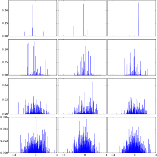
In probability theory, Dirichlet processes are a family of stochastic processes whose realizations are probability distributions. In other words, a Dirichlet process is a probability distribution whose range is itself a set of probability distributions. It is often used in Bayesian inference to describe the prior knowledge about the distribution of random variables—how likely it is that the random variables are distributed according to one or another particular distribution.

In probability and statistics, a natural exponential family (NEF) is a class of probability distributions that is a special case of an exponential family (EF).

In probability theory and statistics, a categorical distribution is a discrete probability distribution that describes the possible results of a random variable that can take on one of K possible categories, with the probability of each category separately specified. There is no innate underlying ordering of these outcomes, but numerical labels are often attached for convenience in describing the distribution,. The K-dimensional categorical distribution is the most general distribution over a K-way event; any other discrete distribution over a size-K sample space is a special case. The parameters specifying the probabilities of each possible outcome are constrained only by the fact that each must be in the range 0 to 1, and all must sum to 1.

In statistical inference, the concept of a confidence distribution (CD) has often been loosely referred to as a distribution function on the parameter space that can represent confidence intervals of all levels for a parameter of interest. Historically, it has typically been constructed by inverting the upper limits of lower sided confidence intervals of all levels, and it was also commonly associated with a fiducial interpretation, although it is a purely frequentist concept. A confidence distribution is NOT a probability distribution function of the parameter of interest, but may still be a function useful for making inferences.

The optical metric was defined by German theoretical physicist Walter Gordon in 1923 to study the geometrical optics in curved space-time filled with moving dielectric materials.

In statistics, the class of vector generalized linear models (VGLMs) was proposed to enlarge the scope of models catered for by generalized linear models (GLMs). In particular, VGLMs allow for response variables outside the classical exponential family and for more than one parameter. Each parameter can be transformed by a link function. The VGLM framework is also large enough to naturally accommodate multiple responses; these are several independent responses each coming from a particular statistical distribution with possibly different parameter values.

A proper reference frame in the theory of relativity is a particular form of accelerated reference frame, that is, a reference frame in which an accelerated observer can be considered as being at rest. It can describe phenomena in curved spacetime, as well as in "flat" Minkowski spacetime in which the spacetime curvature caused by the energy–momentum tensor can be disregarded. Since this article considers only flat spacetime—and uses the definition that special relativity is the theory of flat spacetime while general relativity is a theory of gravitation in terms of curved spacetime—it is consequently concerned with accelerated frames in special relativity.

The hyperbolastic functions, also known as hyperbolastic growth models, are mathematical functions that are used in medical statistical modeling. These models were originally developed to capture the growth dynamics of multicellular tumor spheres, and were introduced in 2005 by Mohammad Tabatabai, David Williams, and Zoran Bursac. The precision of hyperbolastic functions in modeling real world problems is somewhat due to their flexibility in their point of inflection. These functions can be used in a wide variety of modeling problems such as tumor growth, stem cell proliferation, pharma kinetics, cancer growth, sigmoid activation function in neural networks, and epidemiological disease progression or regression.

References

↑ "Posterior Predictive Distribution". SAS. Retrieved 19 July 2014.
↑ Gelman, Andrew; Carlin, John B.; Stern, Hal S.; Dunson, David B.; Vehtari, Aki; Rubin, Donald B. (2013). Bayesian Data Analysis (Third ed.). Chapman and Hall/CRC. p. 7. ISBN 978-1-4398-4095-5.