Linear algebra is the branch of mathematics concerning linear equations such as:
In linear algebra, the rank of a matrix A is the dimension of the vector space generated by its columns. This corresponds to the maximal number of linearly independent columns of A. This, in turn, is identical to the dimension of the vector space spanned by its rows. Rank is thus a measure of the "nondegenerateness" of the system of linear equations and linear transformation encoded by A. There are multiple equivalent definitions of rank. A matrix's rank is one of its most fundamental characteristics.

A dot matrix is a 2-dimensional patterned array, used to represent characters, symbols and images. Most types of modern technology use dot matrices for display of information, including mobile phones, televisions, and printers. The system is also used in textiles with sewing, knitting and weaving.

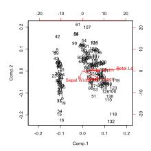
Principal component analysis (PCA) is a linear dimensionality reduction technique with applications in exploratory data analysis, visualization and data preprocessing.

In mathematics, specifically in linear algebra, matrix multiplication is a binary operation that produces a matrix from two matrices. For matrix multiplication, the number of columns in the first matrix must be equal to the number of rows in the second matrix. The resulting matrix, known as the matrix product, has the number of rows of the first and the number of columns of the second matrix. The product of matrices A and B is denoted as AB.

In linear algebra, the singular value decomposition (SVD) is a factorization of a real or complex matrix into a rotation, followed by a rescaling followed by another rotation. It generalizes the eigendecomposition of a square normal matrix with an orthonormal eigenbasis to any matrix. It is related to the polar decomposition.
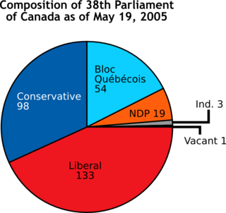
A chart is a graphical representation for data visualization, in which "the data is represented by symbols, such as bars in a bar chart, lines in a line chart, or slices in a pie chart". A chart can represent tabular numeric data, functions or some kinds of quality structure and provides different info.
In linear algebra, the transpose of a matrix is an operator which flips a matrix over its diagonal; that is, it switches the row and column indices of the matrix A by producing another matrix, often denoted by AT.

In probability theory and statistics, a covariance matrix is a square matrix giving the covariance between each pair of elements of a given random vector.
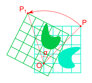
Rotation in mathematics is a concept originating in geometry. Any rotation is a motion of a certain space that preserves at least one point. It can describe, for example, the motion of a rigid body around a fixed point. Rotation can have a sign (as in the sign of an angle): a clockwise rotation is a negative magnitude so a counterclockwise turn has a positive magnitude. A rotation is different from other types of motions: translations, which have no fixed points, and (hyperplane) reflections, each of them having an entire (n − 1)-dimensional flat of fixed points in a n-dimensional space.

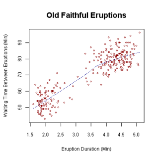
A scatter plot, also called a scatterplot, scatter graph, scatter chart, scattergram, or scatter diagram, is a type of plot or mathematical diagram using Cartesian coordinates to display values for typically two variables for a set of data. If the points are coded (color/shape/size), one additional variable can be displayed. The data are displayed as a collection of points, each having the value of one variable determining the position on the horizontal axis and the value of the other variable determining the position on the vertical axis.
In linear algebra, a rotation matrix is a transformation matrix that is used to perform a rotation in Euclidean space. For example, using the convention below, the matrix
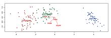
Partial least squares (PLS) regression is a statistical method that bears some relation to principal components regression; instead of finding hyperplanes of maximum variance between the response and independent variables, it finds a linear regression model by projecting the predicted variables and the observable variables to a new space. Because both the X and Y data are projected to new spaces, the PLS family of methods are known as bilinear factor models. Partial least squares discriminant analysis (PLS-DA) is a variant used when the Y is categorical.
The computer graphics pipeline, also known as the rendering pipeline, or graphics pipeline, is a framework within computer graphics that outlines the necessary procedures for transforming a three-dimensional (3D) scene into a two-dimensional (2D) representation on a screen. Once a 3D model is generated, the graphics pipeline converts the model into a visually perceivable format on the computer display. Due to the dependence on specific software, hardware configurations, and desired display attributes, a universally applicable graphics pipeline does not exist. Nevertheless, graphics application programming interfaces (APIs), such as Direct3D, OpenGL and Vulkan were developed to standardize common procedures and oversee the graphics pipeline of a given hardware accelerator. These APIs provide an abstraction layer over the underlying hardware, relieving programmers from the need to write code explicitly targeting various graphics hardware accelerators like AMD, Intel, Nvidia, and others.
In linear algebra, an eigenvector or characteristic vector is a vector that has its direction unchanged by a given linear transformation. More precisely, an eigenvector, , of a linear transformation, , is scaled by a constant factor, , when the linear transformation is applied to it: . It is often important to know these vectors in linear algebra. The corresponding eigenvalue, characteristic value, or characteristic root is the multiplying factor .
Correspondence analysis (CA) is a multivariate statistical technique proposed by Herman Otto Hartley (Hirschfeld) and later developed by Jean-Paul Benzécri. It is conceptually similar to principal component analysis, but applies to categorical rather than continuous data. In a similar manner to principal component analysis, it provides a means of displaying or summarising a set of data in two-dimensional graphical form. Its aim is to display in a biplot any structure hidden in the multivariate setting of the data table. As such it is a technique from the field of multivariate ordination. Since the variant of CA described here can be applied either with a focus on the rows or on the columns it should in fact be called simple (symmetric) correspondence analysis.
A plot is a graphical technique for representing a data set, usually as a graph showing the relationship between two or more variables. The plot can be drawn by hand or by a computer. In the past, sometimes mechanical or electronic plotters were used. Graphs are a visual representation of the relationship between variables, which are very useful for humans who can then quickly derive an understanding which may not have come from lists of values. Given a scale or ruler, graphs can also be used to read off the value of an unknown variable plotted as a function of a known one, but this can also be done with data presented in tabular form. Graphs of functions are used in mathematics, sciences, engineering, technology, finance, and other areas.

In mathematics, a matrix is a rectangular array or table of numbers, symbols, or expressions, with elements or entries arranged in rows and columns, which is used to represent a mathematical object or property of such an object.
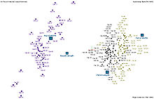
In statistics, multiple correspondence analysis (MCA) is a data analysis technique for nominal categorical data, used to detect and represent underlying structures in a data set. It does this by representing data as points in a low-dimensional Euclidean space. The procedure thus appears to be the counterpart of principal component analysis for categorical data. MCA can be viewed as an extension of simple correspondence analysis (CA) in that it is applicable to a large set of categorical variables.
A CUR matrix approximation is a set of three matrices that, when multiplied together, closely approximate a given matrix. A CUR approximation can be used in the same way as the low-rank approximation of the singular value decomposition (SVD). CUR approximations are less accurate than the SVD, but they offer two key advantages, both stemming from the fact that the rows and columns come from the original matrix :