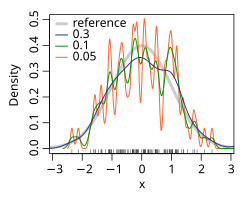
Demonstration of density estimation using Kernel density estimation: The true density is a mixture of two Gaussians centered around 0 and 3, shown with a solid blue curve. In each frame, 100 samples are generated from the distribution, shown in red. Centered on each sample, a Gaussian kernel is drawn in gray. Averaging the Gaussians yields the density estimate shown in the dashed black curve.
In statistics, probability density estimation or simply density estimation is the construction of an estimate, based on observed data, of an unobservable underlying probability density function. The unobservable density function is thought of as the density according to which a large population is distributed; the data are usually thought of as a random sample from that population.[1]
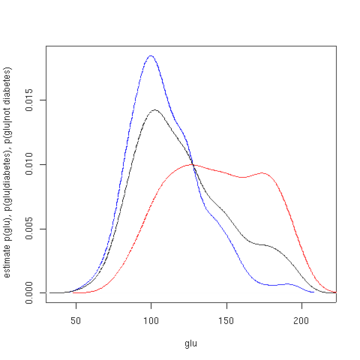
Estimated density of p (glu | diabetes=1) (red), p(glu | diabetes=0) (blue), and p(glu) (black)Estimated probability of p(diabetes=1 | glu)Estimated probability of p(diabetes=1 | glu)
We will consider records of the incidence of diabetes. The following is quoted verbatim from the data set description:
A population of women who were at least 21 years old, of Pima Indian heritage and living near Phoenix, Arizona, was tested for diabetes mellitus according to World Health Organization criteria. The data were collected by the US National Institute of Diabetes and Digestive and Kidney Diseases. We used the 532 complete records.[2][3]
In this example, we construct three density estimates for "glu" (plasmaglucose concentration), one conditional on the presence of diabetes, the second conditional on the absence of diabetes, and the third not conditional on diabetes. The conditional density estimates are then used to construct the probability of diabetes conditional on "glu".
The "glu" data were obtained from the MASS package[4] of the R programming language. Within R, ?Pima.tr and ?Pima.te give a fuller account of the data.
The mean of "glu" in the diabetes cases is 143.1 and the standard deviation is 31.26. The mean of "glu" in the non-diabetes cases is 110.0 and the standard deviation is 24.29. From this we see that, in this data set, diabetes cases are associated with greater levels of "glu". This will be made clearer by plots of the estimated density functions.
The first figure shows density estimates of p(glu | diabetes=1), p(glu | diabetes=0), and p(glu). The density estimates are kernel density estimates using a Gaussian kernel. That is, a Gaussian density function is placed at each data point, and the sum of the density functions is computed over the range of the data.
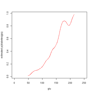
From the density of "glu" conditional on diabetes, we can obtain the probability of diabetes conditional on "glu" via Bayes' rule. For brevity, "diabetes" is abbreviated "db." in this formula.
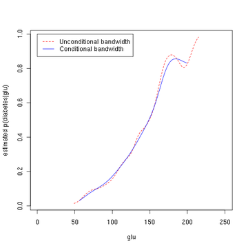
The second figure shows the estimated posterior probability p(diabetes=1 | glu). From these data, it appears that an increased level of "glu" is associated with diabetes.
Application and purpose
A very natural use of density estimates is in the informal investigation of the properties of a given set of data. Density estimates can give a valuable indication of such features as skewness and multimodality in the data. In some cases they will yield conclusions that may then be regarded as self-evidently true, while in others all they will do is to point the way to further analysis and/or data collection.[5]
Histogram and density function for a Gumbel distribution
An important aspect of statistics is often the presentation of data back to the client in order to provide explanation and illustration of conclusions that may possibly have been obtained by other means. Density estimates are ideal for this purpose, for the simple reason that they are fairly easily comprehensible to non-mathematicians.
More examples illustrating the use of density estimates for exploratory and presentational purposes, including the important case of bivariate data.[7]
Density estimation is also frequently used in anomaly detection or novelty detection:[8] if an observation lies in a very low-density region, it is likely to be an anomaly or a novelty.
In hydrology the histogram and estimated density function of rainfall and river discharge data, analysed with a probability distribution, are used to gain insight in their behaviour and frequency of occurrence.[9] An example is shown in the blue figure.
↑ Alberto Bernacchia, Simone Pigolotti, Self-Consistent Method for Density Estimation, Journal of the Royal Statistical Society Series B: Statistical Methodology, Volume 73, Issue 3, June 2011, Pages 407–422, https://doi.org/10.1111/j.1467-9868.2011.00772.x
↑ Pimentel, Marco A.F.; Clifton, David A.; Clifton, Lei; Tarassenko, Lionel (2 January 2014). "A review of novelty detection". Signal Processing. 99 (June 2014): 215–249. doi:10.1016/j.sigpro.2013.12.026.
This page is based on this Wikipedia article Text is available under the CC BY-SA 4.0 license; additional terms may apply. Images, videos and audio are available under their respective licenses.