Multivariate analysis of variance

The image above depicts a visual comparison between multivariate analysis of variance (MANOVA) and univariate analysis of variance (ANOVA). In MANOVA, researchers are examining the group differences of a singular independent variable across multiple outcome variables, whereas in an ANOVA, researchers are examining the group differences of sometimes multiple independent variables on a singular outcome variable. In the provided example, the levels of the IV might include high school, college, and graduate school. The results of a MANOVA can tell us whether an individual who completed graduate school showed higher life AND job satisfaction than an individual who completed only high school or college. Results of an ANOVA can only tell us this information for life satisfaction. Analyzing group differences across multiple outcome variables often provides more accurate information as a pure relationship between only X and only Y rarely exists in nature.

In statistics, multivariate analysis of variance (MANOVA) is a procedure for comparing multivariate sample means. As a multivariate procedure, it is used when there are two or more dependent variables, ^[1] and is often followed by significance tests involving individual dependent variables separately. ^[2]

Without relation to the image, the dependent variables may be k life satisfactions scores measured at sequential time points and p job satisfaction scores measured at sequential time points. In this case there are k+p dependent variables whose linear combination follows a multivariate normal distribution, multivariate variance-covariance matrix homogeneity, and linear relationship, no multicollinearity, and each without outliers.

Model

Assume ${\textstyle n}$${\textstyle q}$-dimensional observations, where the ${\textstyle i}$’th observation ${\textstyle y_{i}}$ is assigned to the group ${\textstyle g(i)\in \{1,\dots ,m\}}$ and is distributed around the group center ${\textstyle \mu ^{(g(i))}\in \mathbb {R} ^{q}}$ with multivariate Gaussian noise: $${\displaystyle y_{i}=\mu ^{(g(i))}+\varepsilon _{i}\quad \varepsilon _{i}{\overset {\text{i.i.d.}}{\sim }}{\mathcal {N}}_{q}(0,\Sigma )\quad {\text{ for }}i=1,\dots ,n,}$$ where ${\textstyle \Sigma }$ is the covariance matrix. Then we formulate our null hypothesis as $${\displaystyle H_{0}\!:\;\mu ^{(1)}=\mu ^{(2)}=\dots =\mu ^{(m)}.}$$

Relationship with ANOVA

MANOVA is a generalized form of univariate analysis of variance (ANOVA), ^[1] although, unlike univariate ANOVA, it uses the covariance between outcome variables in testing the statistical significance of the mean differences.

Where sums of squares appear in univariate analysis of variance, in multivariate analysis of variance certain positive-definite matrices appear. The diagonal entries are the same kinds of sums of squares that appear in univariate ANOVA. The off-diagonal entries are corresponding sums of products. Under normality assumptions about error distributions, the counterpart of the sum of squares due to error has a Wishart distribution.

Hypothesis Testing

First, define the following ${\textstyle n\times q}$ matrices:

• ${\textstyle Y}$: where the ${\textstyle i}$-th row is equal to ${\textstyle y_{i}}$

• ${\textstyle {\hat {Y}}}$: where the ${\textstyle i}$-th row is the best prediction given the group membership ${\textstyle g(i)}$. That is the mean over all observation in group ${\textstyle g(i)}$: ${\textstyle {\frac {1}{{\text{size of group }}g(i)}}\sum _{k:g(k)=g(i)}y_{k}}$.

• ${\textstyle {\bar {Y}}}$: where the ${\textstyle i}$-th row is the best prediction given no information. That is the empirical mean over all ${\textstyle n}$ observations ${\textstyle {\frac {1}{n}}\sum _{k=1}^{n}y_{k}}$

Then the matrix ${\textstyle S_{\text{model}}:=({\hat {Y}}-{\bar {Y}})^{T}({\hat {Y}}-{\bar {Y}})}$ is a generalization of the sum of squares explained by the group, and ${\textstyle S_{\text{res}}:=(Y-{\hat {Y}})^{T}(Y-{\hat {Y}})}$ is a generalization of the residual sum of squares. ^{[3] [4]} Note that alternatively one could also speak about covariances when the abovementioned matrices are scaled by 1/(n-1) since the subsequent test statistics do not change by multiplying ${\textstyle S_{\text{model}}}$ and ${\textstyle S_{\text{res}}}$ by the same non-zero constant.

The most common ^{[3] [5]} statistics are summaries based on the roots (or eigenvalues) ${\textstyle \lambda _{p}}$ of the matrix ${\textstyle A:=S_{\text{model}}S_{\text{res}}^{-1}}$

• Samuel Stanley Wilks' ${\displaystyle \Lambda _{\text{Wilks}}=\prod _{1,\ldots ,p}(1/(1+\lambda _{p}))=\det(I+A)^{-1}=\det(S_{\text{res}})/\det(S_{\text{res}}+S_{\text{model}})}$ distributed as lambda (Λ)
• the K. C. Sreedharan Pillai–M. S. Bartlett trace, ${\displaystyle \Lambda _{\text{Pillai}}=\sum _{1,\ldots ,p}(\lambda _{p}/(1+\lambda _{p}))=\operatorname {tr} (A(I+A)^{-1})}$ ^[6]
• the Lawley–Hotelling trace, ${\displaystyle \Lambda _{\text{LH}}=\sum _{1,\ldots ,p}(\lambda _{p})=\operatorname {tr} (A)}$
• Roy's greatest root (also called Roy's largest root), ${\displaystyle \Lambda _{\text{Roy}}=\max _{p}(\lambda _{p})}$

Discussion continues over the merits of each, ^[1] although the greatest root leads only to a bound on significance which is not generally of practical interest. A further complication is that, except for the Roy's greatest root, the distribution of these statistics under the null hypothesis is not straightforward and can only be approximated except in a few low-dimensional cases. An algorithm for the distribution of the Roy's largest root under the null hypothesis was derived in ^[7] while the distribution under the alternative is studied in. ^[8]

The best-known approximation for Wilks' lambda was derived by C. R. Rao.

In the case of two groups, all the statistics are equivalent and the test reduces to Hotelling's T-square.

Introducing covariates (MANCOVA)

Main article: Multivariate analysis of covariance

One can also test if there is a group effect after adjusting for covariates. For this, follow the procedure above but substitute ${\textstyle {\hat {Y}}}$ with the predictions of the general linear model, containing the group and the covariates, and substitute ${\textstyle {\bar {Y}}}$ with the predictions of the general linear model containing only the covariates (and an intercept). Then ${\textstyle S_{\text{model}}}$ are the additional sum of squares explained by adding the grouping information and ${\textstyle S_{\text{res}}}$ is the residual sum of squares of the model containing the grouping and the covariates. ^[4]

Note that in case of unbalanced data, the order of adding the covariates matter.

Correlation of dependent variables

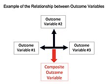
This is a graphical depiction of the required relationship amongst outcome variables in a multivariate analysis of variance. Part of the analysis involves creating a composite variable, which the group differences of the independent variable are analyzed against. The composite variables, as there can be multiple, are different combinations of the outcome variables. The analysis then determines which combination shows the greatest group differences for the independent variable. A descriptive discriminant analysis is then used as a post hoc test to determine what the makeup of that composite variable is that creates the greatest group differences.

This is a simple visual representation of the effect of two highly correlated dependent variables within a MANOVA. If two (or more) dependent variables are highly correlated, the chances of a Type I error occurring is reduced, but the trade-off is that the power of the MANOVA test is also reduced.

MANOVA's power is affected by the correlations of the dependent variables and by the effect sizes associated with those variables. For example, when there are two groups and two dependent variables, MANOVA's power is lowest when the correlation equals the ratio of the smaller to the larger standardized effect size. ^[9]

See also

• Permutational analysis of variance for a non-parametric alternative
• Discriminant function analysis
• Canonical correlation analysis
• Multivariate analysis of variance (Wikiversity)
• Repeated measures design

References

1. Warne, R. T. (2014). "A primer on multivariate analysis of variance (MANOVA) for behavioral scientists". Practical Assessment, Research & Evaluation. 19 (17): 1–10.
2. Stevens, J. P. (2002). Applied multivariate statistics for the social sciences. Mahwah, NJ: Lawrence Erblaum.
3. Anderson, T. W. (1994). An Introduction to Multivariate Statistical Analysis. Wiley.
4. Krzanowski, W. J. (1988). Principles of Multivariate Analysis. A User's Perspective. Oxford University Press.
5. UCLA: Academic Technology Services, Statistical Consulting Group. "Stata Annotated Output – MANOVA" . Retrieved 2024-02-10.
6. "MANOVA Basic Concepts – Real Statistics Using Excel". www.real-statistics.com. Retrieved 5 April 2018.
7. Chiani, M. (2016), "Distribution of the largest root of a matrix for Roy's test in multivariate analysis of variance", Journal of Multivariate Analysis , 143: 467–471, arXiv: 1401.3987v3 , doi:10.1016/j.jmva.2015.10.007, S2CID   37620291
8. I.M. Johnstone, B. Nadler "Roy's largest root test under rank-one alternatives" arXiv preprint arXiv:1310.6581 (2013)
9. Frane, Andrew (2015). "Power and Type I Error Control for Univariate Comparisons in Multivariate Two-Group Designs". Multivariate Behavioral Research. 50 (2): 233–247. doi:10.1080/00273171.2014.968836. PMID   26609880. S2CID   1532673.