Repeated measures design

Last updated

Repeated measures design is a research design that involves multiple measures of the same variable taken on the same or matched subjects either under different conditions or over two or more time periods. [1] For instance, repeated measurements are collected in a longitudinal study in which change over time is assessed.

Contents

Crossover studies

A popular repeated-measures design is the crossover study. A crossover study is a longitudinal study in which subjects receive a sequence of different treatments (or exposures). While crossover studies can be observational studies, many important crossover studies are controlled experiments. Crossover designs are common for experiments in many scientific disciplines, for example psychology, education, pharmaceutical science, and health care, especially medicine.

Randomized, controlled, crossover experiments are especially important in health care. In a randomized clinical trial, the subjects are randomly assigned treatments. When such a trial is a repeated measures design, the subjects are randomly assigned to a sequence of treatments. A crossover clinical trial is a repeated-measures design in which each patient is randomly assigned to a sequence of treatments, including at least two treatments (of which one may be a standard treatment or a placebo): Thus each patient crosses over from one treatment to another.

Nearly all crossover designs have "balance", which means that all subjects should receive the same number of treatments and that all subjects participate for the same number of periods. In most crossover trials, each subject receives all treatments.

However, many repeated-measures designs are not crossovers: the longitudinal study of the sequential effects of repeated treatments need not use any "crossover", for example (Vonesh & Chinchilli; Jones & Kenward).

Uses

Order effects

Order effects may occur when a participant in an experiment is able to perform a task and then perform it again. Examples of order effects include performance improvement or decline in performance, which may be due to learning effects, boredom or fatigue. The impact of order effects may be smaller in long-term longitudinal studies or by counterbalancing using a crossover design.

Counterbalancing

In this technique, two groups each perform the same tasks or experience the same conditions, but in reverse order. With two tasks or conditions, four groups are formed.

Counterbalancing
Task/ConditionTask/ConditionRemarks
Group A
1
2
Group A performs Task/Condition 1 first, then Task/Condition 2
Group B
2
1
Group B performs Task/Condition 2 first, then Task/Condition 1

Counterbalancing attempts to take account of two important sources of systematic variation in this type of design: practice and boredom effects. Both might otherwise lead to different performance of participants due to familiarity with or tiredness to the treatments.

Limitations

It may not be possible for each participant to be in all conditions of the experiment (i.e. time constraints, location of experiment, etc.). Severely diseased subjects tend to drop out of longitudinal studies, potentially biasing the results. In these cases mixed effects models would be preferable as they can deal with missing values.

Mean regression may affect conditions with significant repetitions. Maturation may affect studies that extend over time. Events outside the experiment may change the response between repetitions.

Repeated measures ANOVA

This figure is an example of a repeated measures design that could be analyzed using a rANOVA (repeated measures ANOVA). The independent variable is the time (Levels: Time 1, Time 2, Time 3, Time 4) that someone took the measure, and the dependent variable is the happiness measure score. Example participant happiness scores are provided for 3 participants for each time or level of the independent variable. Repeated Measures ANOVA Example.png
This figure is an example of a repeated measures design that could be analyzed using a rANOVA (repeated measures ANOVA). The independent variable is the time (Levels: Time 1, Time 2, Time 3, Time 4) that someone took the measure, and the dependent variable is the happiness measure score. Example participant happiness scores are provided for 3 participants for each time or level of the independent variable.

Repeated measures analysis of variance (rANOVA) is a commonly used statistical approach to repeated measure designs. [3] With such designs, the repeated-measure factor (the qualitative independent variable) is the within-subjects factor, while the dependent quantitative variable on which each participant is measured is the dependent variable.

Partitioning of error

One of the greatest advantages to rANOVA, as is the case with repeated measures designs in general, is the ability to partition out variability due to individual differences. Consider the general structure of the F-statistic:

F = MSTreatment / MSError = (SSTreatment/dfTreatment)/(SSError/dfError)

In a between-subjects design there is an element of variance due to individual difference that is combined with the treatment and error terms:

SSTotal = SSTreatment + SSError
dfTotal = n − 1

In a repeated measures design it is possible to partition subject variability from the treatment and error terms. In such a case, variability can be broken down into between-treatments variability (or within-subjects effects, excluding individual differences) and within-treatments variability. The within-treatments variability can be further partitioned into between-subjects variability (individual differences) and error (excluding the individual differences): [4]

SSTotal = SSTreatment (excluding individual difference) + SSSubjects + SSError
dfTotal = dfTreatment (within subjects) + dfbetween subjects + dferror = (k − 1) + (n − 1) + ((nk)(n − 1))

In reference to the general structure of the F-statistic, it is clear that by partitioning out the between-subjects variability, the F-value will increase because the sum of squares error term will be smaller resulting in a smaller MSError. It is noteworthy that partitioning variability reduces degrees of freedom from the F-test, therefore the between-subjects variability must be significant enough to offset the loss in degrees of freedom. If between-subjects variability is small this process may actually reduce the F-value. [4]

Assumptions

As with all statistical analyses, specific assumptions should be met to justify the use of this test. Violations can moderately to severely affect results and often lead to an inflation of type 1 error. With the rANOVA, standard univariate and multivariate assumptions apply. [5] The univariate assumptions are:

The rANOVA also requires that certain multivariate assumptions be met, because a multivariate test is conducted on difference scores. These assumptions include:

F test

As with other analysis of variance tests, the rANOVA makes use of an F statistic to determine significance. Depending on the number of within-subjects factors and assumption violations, it is necessary to select the most appropriate of three tests: [5]

Effect size

One of the most commonly reported effect size statistics for rANOVA is partial eta-squared (ηp2). It is also common to use the multivariate η2 when the assumption of sphericity has been violated, and the multivariate test statistic is reported. A third effect size statistic that is reported is the generalized η2, which is comparable to ηp2 in a one-way repeated measures ANOVA. It has been shown to be a better estimate of effect size with other within-subjects tests. [8] [9]

Cautions

rANOVA is not always the best statistical analysis for repeated measure designs. The rANOVA is vulnerable to effects from missing values, imputation, unequivalent time points between subjects and violations of sphericity. [3] These issues can result in sampling bias and inflated rates of Type I error. [10] In such cases it may be better to consider use of a linear mixed model. [11]

See also

Notes

  1. Kraska; Marie (2010), "Repeated Measures Design", Encyclopedia of Research Design, California, USA: SAGE Publications, Inc., doi:10.4135/9781412961288.n378, ISBN   978-1-4129-6127-1, S2CID   149337088
  2. Barret, Julia R. (2013). "Particulate Matter and Cardiovascular Disease: Researchers Turn an Eye toward Microvascular Changes". Environmental Health Perspectives. 121 (9): a282. doi:10.1289/ehp.121-A282. PMC   3764084 . PMID   24004855.
  3. 1 2 Gueorguieva; Krystal (2004). "Move Over ANOVA". Arch Gen Psychiatry. 61 (3): 310–7. doi:10.1001/archpsyc.61.3.310. PMID   14993119.
  4. 1 2 Howell, David C. (2010). Statistical methods for psychology (7th ed.). Belmont, CA: Thomson Wadsworth. ISBN   978-0-495-59784-1.
  5. 1 2 Salkind, Samuel B. Green, Neil J. (2011). Using SPSS for Windows and Macintosh : analyzing and understanding data (6th ed.). Boston: Prentice Hall. ISBN   978-0-205-02040-9.{{cite book}}: CS1 maint: multiple names: authors list (link)
  6. Vasey; Thayer (1987). "The Continuing Problem of False Positives in Repeated Measures ANOVA in Psychophysiology: A Multivariate Solution". Psychophysiology. 24 (4): 479–486. doi:10.1111/j.1469-8986.1987.tb00324.x. PMID   3615759.
  7. Park (1993). "A comparison of the generalized estimating equation approach with the maximum likelihood approach for repeated measurements". Stat Med. 12 (18): 1723–1732. doi:10.1002/sim.4780121807. PMID   8248664.
  8. Bakeman (2005). "Recommended effect size statistics for repeated measures designs". Behavior Research Methods. 37 (3): 379–384. doi: 10.3758/bf03192707 . PMID   16405133.
  9. Olejnik; Algina (2003). "Generalized eta and omega squared statistics: Measures of effect size for some common research designs". Psychological Methods. 8 (4): 434–447. doi:10.1037/1082-989x.8.4.434. PMID   14664681. S2CID   6931663.
  10. Muller; Barton (1989). "Approximate Power for Repeated-Measures ANOVA lacking sphericity". Journal of the American Statistical Association. 84 (406): 549–555. doi:10.1080/01621459.1989.10478802.
  11. Kreuger; Tian (2004). "A comparison of the general linear mixed model and repeated measures ANOVA using a dataset with multiple missing data points". Biological Research for Nursing. 6 (2): 151–157. doi:10.1177/1099800404267682. PMID   15388912. S2CID   23173349.

Related Research Articles

Analysis of variance (ANOVA) is a collection of statistical models and their associated estimation procedures used to analyze the differences among means. ANOVA was developed by the statistician Ronald Fisher. ANOVA is based on the law of total variance, where the observed variance in a particular variable is partitioned into components attributable to different sources of variation. In its simplest form, ANOVA provides a statistical test of whether two or more population means are equal, and therefore generalizes the t-test beyond two means. In other words, the ANOVA is used to test the difference between two or more means.

<i>F</i>-test Statistical hypothesis test, mostly using multiple restrictions

An F-test is any statistical test used to compare the variances of two samples or the ratio of variances between multiple samples. The test statistic, random variable F, is used to determine if the tested data has an F-distribution under the true null hypothesis, and true customary assumptions about the error term (ε). It is most often used when comparing statistical models that have been fitted to a data set, in order to identify the model that best fits the population from which the data were sampled. Exact "F-tests" mainly arise when the models have been fitted to the data using least squares. The name was coined by George W. Snedecor, in honour of Ronald Fisher. Fisher initially developed the statistic as the variance ratio in the 1920s.

Analysis of covariance (ANCOVA) is a general linear model that blends ANOVA and regression. ANCOVA evaluates whether the means of a dependent variable (DV) are equal across levels of one or more categorical independent variables (IV) and across one or more continuous variables. For example, the categorical variable(s) might describe treatment and the continuous variable(s) might be covariates or nuisance variables; or vice versa. Mathematically, ANCOVA decomposes the variance in the DV into variance explained by the CV(s), variance explained by the categorical IV, and residual variance. Intuitively, ANCOVA can be thought of as 'adjusting' the DV by the group means of the CV(s).

<span class="mw-page-title-main">Multivariate analysis of variance</span> Procedure for comparing multivariate sample means

In statistics, multivariate analysis of variance (MANOVA) is a procedure for comparing multivariate sample means. As a multivariate procedure, it is used when there are two or more dependent variables, and is often followed by significance tests involving individual dependent variables separately.

<span class="mw-page-title-main">Mathematical statistics</span> Branch of statistics

Mathematical statistics is the application of probability theory, a branch of mathematics, to statistics, as opposed to techniques for collecting statistical data. Specific mathematical techniques which are used for this include mathematical analysis, linear algebra, stochastic analysis, differential equations, and measure theory.

In medicine, a crossover study or crossover trial is a longitudinal study in which subjects receive a sequence of different treatments. While crossover studies can be observational studies, many important crossover studies are controlled experiments, which are discussed in this article. Crossover designs are common for experiments in many scientific disciplines, for example psychology, pharmaceutical science, and medicine.

Multilevel models are statistical models of parameters that vary at more than one level. An example could be a model of student performance that contains measures for individual students as well as measures for classrooms within which the students are grouped. These models can be seen as generalizations of linear models, although they can also extend to non-linear models. These models became much more popular after sufficient computing power and software became available.

A mixed model, mixed-effects model or mixed error-component model is a statistical model containing both fixed effects and random effects. These models are useful in a wide variety of disciplines in the physical, biological and social sciences. They are particularly useful in settings where repeated measurements are made on the same statistical units, or where measurements are made on clusters of related statistical units. Mixed models are often preferred over traditional analysis of variance regression models because they don't rely on the independent observations assumption. Further, they have their flexibility in dealing with missing values and uneven spacing of repeated measurements. The Mixed model analysis allows measurements to be explicitly modeled in a wider variety of correlation and variance-covariance avoiding biased estimations. structures.

<span class="mw-page-title-main">Pseudoreplication</span>

Pseudoreplication has many definitions. Pseudoreplication was originally defined in 1984 by Stuart H. Hurlbert as the use of inferential statistics to test for treatment effects with data from experiments where either treatments are not replicated or replicates are not statistically independent. Subsequently, Millar and Anderson identified it as a special case of inadequate specification of random factors where both random and fixed factors are present. It is sometimes narrowly interpreted as an inflation of the number of samples or replicates which are not statistically independent. This definition omits the confounding of unit and treatment effects in a misspecified F-ratio. In practice, incorrect F-ratios for statistical tests of fixed effects often arise from a default F-ratio that is formed over the error rather the mixed term.

Mauchly's sphericity test or Mauchly's W is a statistical test used to validate a repeated measures analysis of variance (ANOVA). It was developed in 1940 by John Mauchly.

In statistics, one-way analysis of variance is a technique to compare whether two or more samples' means are significantly different. This analysis of variance technique requires a numeric response variable "Y" and a single explanatory variable "X", hence "one-way".

Multivariate analysis of covariance (MANCOVA) is an extension of analysis of covariance (ANCOVA) methods to cover cases where there is more than one dependent variable and where the control of concomitant continuous independent variables – covariates – is required. The most prominent benefit of the MANCOVA design over the simple MANOVA is the 'factoring out' of noise or error that has been introduced by the covariant. A commonly used multivariate version of the ANOVA F-statistic is Wilks' Lambda (Λ), which represents the ratio between the error variance and the effect variance.

In statistics, restricted randomization occurs in the design of experiments and in particular in the context of randomized experiments and randomized controlled trials. Restricted randomization allows intuitively poor allocations of treatments to experimental units to be avoided, while retaining the theoretical benefits of randomization. For example, in a clinical trial of a new proposed treatment of obesity compared to a control, an experimenter would want to avoid outcomes of the randomization in which the new treatment was allocated only to the heaviest patients.

In statistics, a mixed-design analysis of variance model, also known as a split-plot ANOVA, is used to test for differences between two or more independent groups whilst subjecting participants to repeated measures. Thus, in a mixed-design ANOVA model, one factor is a between-subjects variable and the other is a within-subjects variable. Thus, overall, the model is a type of mixed-effects model.

In randomized statistical experiments, generalized randomized block designs (GRBDs) are used to study the interaction between blocks and treatments. For a GRBD, each treatment is replicated at least two times in each block; this replication allows the estimation and testing of an interaction term in the linear model.

In statistics, one purpose for the analysis of variance (ANOVA) is to analyze differences in means between groups. The test statistic, F, assumes independence of observations, homogeneous variances, and population normality. ANOVA on ranks is a statistic designed for situations when the normality assumption has been violated.

In statistics, the two-way analysis of variance (ANOVA) is an extension of the one-way ANOVA that examines the influence of two different categorical independent variables on one continuous dependent variable. The two-way ANOVA not only aims at assessing the main effect of each independent variable but also if there is any interaction between them.

One application of multilevel modeling (MLM) is the analysis of repeated measures data. Multilevel modeling for repeated measures data is most often discussed in the context of modeling change over time ; however, it may also be used for repeated measures data in which time is not a factor.
<span class="mw-page-title-main">Homoscedasticity and heteroscedasticity</span> Statistical property

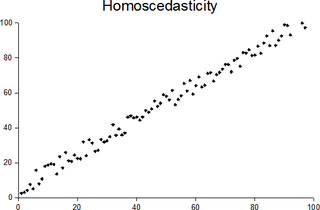
In statistics, a sequence of random variables is homoscedastic if all its random variables have the same finite variance; this is also known as homogeneity of variance. The complementary notion is called heteroscedasticity, also known as heterogeneity of variance. The spellings homoskedasticity and heteroskedasticity are also frequently used. Skedasticity comes from the Ancient Greek word skedánnymi, meaning “to scatter”. Assuming a variable is homoscedastic when in reality it is heteroscedastic results in unbiased but inefficient point estimates and in biased estimates of standard errors, and may result in overestimating the goodness of fit as measured by the Pearson coefficient.

References

Design and analysis of experiments

Exploration of longitudinal data