Econometrics is an application of statistical methods to economic data in order to give empirical content to economic relationships. More precisely, it is "the quantitative analysis of actual economic phenomena based on the concurrent development of theory and observation, related by appropriate methods of inference." An introductory economics textbook describes econometrics as allowing economists "to sift through mountains of data to extract simple relationships." Jan Tinbergen is one of the two founding fathers of econometrics. The other, Ragnar Frisch, also coined the term in the sense in which it is used today.
In statistics, the Gauss–Markov theorem states that the ordinary least squares (OLS) estimator has the lowest sampling variance within the class of linear unbiased estimators, if the errors in the linear regression model are uncorrelated, have equal variances and expectation value of zero. The errors do not need to be normal for the theorem to apply, nor do they need to be independent and identically distributed.
Simultaneous equations models are a type of statistical model in which the dependent variables are functions of other dependent variables, rather than just independent variables. This means some of the explanatory variables are jointly determined with the dependent variable, which in economics usually is the consequence of some underlying equilibrium mechanism. Take the typical supply and demand model: whilst typically one would determine the quantity supplied and demanded to be a function of the price set by the market, it is also possible for the reverse to be true, where producers observe the quantity that consumers demand and then set the price.
In statistics, and particularly in econometrics, the reduced form of a system of equations is the result of solving the system for the endogenous variables. This gives the latter as functions of the exogenous variables, if any. In econometrics, the equations of a structural form model are estimated in their theoretically given form, while an alternative approach to estimation is to first solve the theoretical equations for the endogenous variables to obtain reduced form equations, and then to estimate the reduced form equations.
In statistics, econometrics, epidemiology and related disciplines, the method of instrumental variables (IV) is used to estimate causal relationships when controlled experiments are not feasible or when a treatment is not successfully delivered to every unit in a randomized experiment. Intuitively, IVs are used when an explanatory variable of interest is correlated with the error term (endogenous), in which case ordinary least squares and ANOVA give biased results. A valid instrument induces changes in the explanatory variable but has no independent effect on the dependent variable and is not correlated with the error term, allowing a researcher to uncover the causal effect of the explanatory variable on the dependent variable.
In statistics, omitted-variable bias (OVB) occurs when a statistical model leaves out one or more relevant variables. The bias results in the model attributing the effect of the missing variables to those that were included.
In statistics, ordinary least squares (OLS) is a type of linear least squares method for choosing the unknown parameters in a linear regression model by the principle of least squares: minimizing the sum of the squares of the differences between the observed dependent variable in the input dataset and the output of the (linear) function of the independent variable.
In econometrics, endogeneity broadly refers to situations in which an explanatory variable is correlated with the error term. The distinction between endogenous and exogenous variables originated in simultaneous equations models, where one separates variables whose values are determined by the model from variables which are predetermined. Ignoring simultaneity in the estimation leads to biased estimates as it violates the exogeneity assumption of the Gauss–Markov theorem. The problem of endogeneity is often ignored by researchers conducting non-experimental research and doing so precludes making policy recommendations. Instrumental variable techniques are commonly used to mitigate this problem.
In statistics and econometrics, panel data and longitudinal data are both multi-dimensional data involving measurements over time. Panel data is a subset of longitudinal data where observations are for the same subjects each time.
In econometrics, the seemingly unrelated regressions (SUR) or seemingly unrelated regression equations (SURE) model, proposed by Arnold Zellner in (1962), is a generalization of a linear regression model that consists of several regression equations, each having its own dependent variable and potentially different sets of exogenous explanatory variables. Each equation is a valid linear regression on its own and can be estimated separately, which is why the system is called seemingly unrelated, although some authors suggest that the term seemingly related would be more appropriate, since the error terms are assumed to be correlated across the equations.
Difference in differences is a statistical technique used in econometrics and quantitative research in the social sciences that attempts to mimic an experimental research design using observational study data, by studying the differential effect of a treatment on a 'treatment group' versus a 'control group' in a natural experiment. It calculates the effect of a treatment on an outcome by comparing the average change over time in the outcome variable for the treatment group to the average change over time for the control group. Although it is intended to mitigate the effects of extraneous factors and selection bias, depending on how the treatment group is chosen, this method may still be subject to certain biases.
In statistics, a fixed effects model is a statistical model in which the model parameters are fixed or non-random quantities. This is in contrast to random effects models and mixed models in which all or some of the model parameters are random variables. In many applications including econometrics and biostatistics a fixed effects model refers to a regression model in which the group means are fixed (non-random) as opposed to a random effects model in which the group means are a random sample from a population. Generally, data can be grouped according to several observed factors. The group means could be modeled as fixed or random effects for each grouping. In a fixed effects model each group mean is a group-specific fixed quantity.
In economics, discrete choice models, or qualitative choice models, describe, explain, and predict choices between two or more discrete alternatives, such as entering or not entering the labor market, or choosing between modes of transport. Such choices contrast with standard consumption models in which the quantity of each good consumed is assumed to be a continuous variable. In the continuous case, calculus methods can be used to determine the optimum amount chosen, and demand can be modeled empirically using regression analysis. On the other hand, discrete choice analysis examines situations in which the potential outcomes are discrete, such that the optimum is not characterized by standard first-order conditions. Thus, instead of examining "how much" as in problems with continuous choice variables, discrete choice analysis examines "which one". However, discrete choice analysis can also be used to examine the chosen quantity when only a few distinct quantities must be chosen from, such as the number of vehicles a household chooses to own and the number of minutes of telecommunications service a customer decides to purchase. Techniques such as logistic regression and probit regression can be used for empirical analysis of discrete choice.
In statistics, a random effects model, also called a variance components model, is a statistical model where the model parameters are random variables. It is a kind of hierarchical linear model, which assumes that the data being analysed are drawn from a hierarchy of different populations whose differences relate to that hierarchy. A random effects model is a special case of a mixed model.

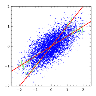
In statistics, errors-in-variables models or measurement error models are regression models that account for measurement errors in the independent variables. In contrast, standard regression models assume that those regressors have been measured exactly, or observed without error; as such, those models account only for errors in the dependent variables, or responses.
In statistics and econometrics, the first-difference (FD) estimator is an estimator used to address the problem of omitted variables with panel data. It is consistent under the assumptions of the fixed effects model. In certain situations it can be more efficient than the standard fixed effects estimator.
In econometrics, the Arellano–Bond estimator is a generalized method of moments estimator used to estimate dynamic models of panel data. It was proposed in 1991 by Manuel Arellano and Stephen Bond, based on the earlier work by Alok Bhargava and John Denis Sargan in 1983, for addressing certain endogeneity problems. The GMM-SYS estimator is a system that contains both the levels and the first difference equations. It provides an alternative to the standard first difference GMM estimator.
In linear panel analysis, it can be desirable to estimate the magnitude of the fixed effects, as they provide measures of the unobserved components. For instance, in wage equation regressions, fixed effects capture unobservables that are constant over time, such as motivation. Chamberlain's approach to unobserved effects models is a way of estimating the linear unobserved effects, under fixed effect assumptions, in the following unobserved effects model
Control functions are statistical methods to correct for endogeneity problems by modelling the endogeneity in the error term. The approach thereby differs in important ways from other models that try to account for the same econometric problem. Instrumental variables, for example, attempt to model the endogenous variable X as an often invertible model with respect to a relevant and exogenous instrument Z. Panel analysis uses special data properties to difference out unobserved heterogeneity that is assumed to be fixed over time.
In statistics, linear regression is a statistical model which estimates the linear relationship between a scalar response and one or more explanatory variables. The case of one explanatory variable is called simple linear regression; for more than one, the process is called multiple linear regression. This term is distinct from multivariate linear regression, where multiple correlated dependent variables are predicted, rather than a single scalar variable. If the explanatory variables are measured with error then errors-in-variables models are required, also known as measurement error models.


