Contingency table

Last updated October 31, 2023

In statistics, a contingency table (also known as a cross tabulation or crosstab) is a type of table in a matrix format that displays the multivariate frequency distribution of the variables. They are heavily used in survey research, business intelligence, engineering, and scientific research. They provide a basic picture of the interrelation between two variables and can help find interactions between them. The term contingency table was first used by Karl Pearson in "On the Theory of Contingency and Its Relation to Association and Normal Correlation",^[1] part of the Drapers' Company Research Memoirs Biometric Series I published in 1904.

A crucial problem of multivariate statistics is finding the (direct-)dependence structure underlying the variables contained in high-dimensional contingency tables. If some of the conditional independences are revealed, then even the storage of the data can be done in a smarter way (see Lauritzen (2002)). In order to do this one can use information theory concepts, which gain the information only from the distribution of probability, which can be expressed easily from the contingency table by the relative frequencies.

A pivot table is a way to create contingency tables using spreadsheet software.

Example

Suppose there are two variables, sex (male or female) and handedness (right- or left-handed). Further suppose that 100 individuals are randomly sampled from a very large population as part of a study of sex differences in handedness. A contingency table can be created to display the numbers of individuals who are male right-handed and left-handed, female right-handed and left-handed. Such a contingency table is shown below.

Handed- ness Sex	Right-handed	Left-handed	Total
Male	43	9	52
Female	44	4	48
Total	87	13	100

The numbers of the males, females, and right- and left-handed individuals are called marginal totals. The grand total (the total number of individuals represented in the contingency table) is the number in the bottom right corner.

The table allows users to see at a glance that the proportion of men who are right-handed is about the same as the proportion of women who are right-handed although the proportions are not identical. The strength of the association can be measured by the odds ratio, and the population odds ratio estimated by the sample odds ratio. The significance of the difference between the two proportions can be assessed with a variety of statistical tests including Pearson's chi-squared test, the G-test, Fisher's exact test, Boschloo's test, and Barnard's test, provided the entries in the table represent individuals randomly sampled from the population about which conclusions are to be drawn. If the proportions of individuals in the different columns vary significantly between rows (or vice versa), it is said that there is a contingency between the two variables. In other words, the two variables are not independent. If there is no contingency, it is said that the two variables are independent.

The example above is the simplest kind of contingency table, a table in which each variable has only two levels; this is called a 2 × 2 contingency table. In principle, any number of rows and columns may be used. There may also be more than two variables, but higher order contingency tables are difficult to represent visually. The relation between ordinal variables, or between ordinal and categorical variables, may also be represented in contingency tables, although such a practice is rare. For more on the use of a contingency table for the relation between two ordinal variables, see Goodman and Kruskal's gamma.

Standard contents of a contingency table

Multiple columns (historically, they were designed to use up all the white space of a printed page). Where each row refers to a specific sub-group in the population (in this case men or women), the columns are sometimes referred to as banner points or cuts (and the rows are sometimes referred to as stubs).
Significance tests. Typically, either column comparisons, which test for differences between columns and display these results using letters, or, cell comparisons, which use color or arrows to identify a cell in a table that stands out in some way.
Nets or netts which are sub-totals.
One or more of: percentages, row percentages, column percentages, indexes or averages.
Unweighted sample sizes (counts).

Measures of association

The degree of association between the two variables can be assessed by a number of coefficients. The following subsections describe a few of them. For a more complete discussion of their uses, see the main articles linked under each subsection heading.

Odds ratio

The simplest measure of association for a 2 × 2 contingency table is the odds ratio. Given two events, A and B, the odds ratio is defined as the ratio of the odds of A in the presence of B and the odds of A in the absence of B, or equivalently (due to symmetry), the ratio of the odds of B in the presence of A and the odds of B in the absence of A. Two events are independent if and only if the odds ratio is 1; if the odds ratio is greater than 1, the events are positively associated; if the odds ratio is less than 1, the events are negatively associated.

The odds ratio has a simple expression in terms of probabilities; given the joint probability distribution:

{\begin{array}{c|cc}&B=1&B=0\\\hline A=1&p_{11}&p_{10}\\A=0&p_{01}&p_{00}\end{array}}

the odds ratio is:

OR={\frac {p_{11}p_{00}}{p_{10}p_{01}}}.

Phi coefficient

A simple measure, applicable only to the case of 2 × 2 contingency tables, is the phi coefficient (φ) defined by

\phi =\pm {\sqrt {\frac {\chi ^{2}}{N}}},

where $χ 2$ is computed as in Pearson's chi-squared test, and N is the grand total of observations. φ varies from 0 (corresponding to no association between the variables) to 1 or −1 (complete association or complete inverse association), provided it is based on frequency data represented in 2 × 2 tables. Then its sign equals the sign of the product of the main diagonal elements of the table minus the product of the off–diagonal elements. φ takes on the minimum value −1.0 or the maximum value of +1.0 if and only if every marginal proportion is equal to 0.5 (and two diagonal cells are empty).^[2]

Cramér's V and the contingency coefficient C

Two alternatives are the contingency coefficientC, and Cramér's V.

The formulae for the C and V coefficients are:

C={\sqrt {\frac {\chi ^{2}}{N+\chi ^{2}}}}

and

V={\sqrt {\frac {\chi ^{2}}{N(k-1)}}},

k being the number of rows or the number of columns, whichever is less.

C suffers from the disadvantage that it does not reach a maximum of 1.0, notably the highest it can reach in a 2 × 2 table is 0.707 . It can reach values closer to 1.0 in contingency tables with more categories; for example, it can reach a maximum of 0.870 in a 4 × 4 table. It should, therefore, not be used to compare associations in different tables if they have different numbers of categories.^[3]

C can be adjusted so it reaches a maximum of 1.0 when there is complete association in a table of any number of rows and columns by dividing C by ${\sqrt {\frac {k-1}{k}}}$ where k is the number of rows or columns, when the table is square ^{[ citation needed ]}, or by ${\sqrt[{\scriptstyle 4}]{{r-1 \over r}\times {c-1 \over c}}}$ where r is the number of rows and c is the number of columns.^[4]

Tetrachoric correlation coefficient

Another choice is the tetrachoric correlation coefficient but it is only applicable to 2 × 2 tables. Polychoric correlation is an extension of the tetrachoric correlation to tables involving variables with more than two levels.

Tetrachoric correlation assumes that the variable underlying each dichotomous measure is normally distributed.^[5] The coefficient provides "a convenient measure of [the Pearson product-moment] correlation when graduated measurements have been reduced to two categories."^[6]

The tetrachoric correlation coefficient should not be confused with the Pearson correlation coefficient computed by assigning, say, values 0.0 and 1.0 to represent the two levels of each variable (which is mathematically equivalent to the φ coefficient).

Lambda coefficient

The lambda coefficient is a measure of the strength of association of the cross tabulations when the variables are measured at the nominal level. Values range from 0.0 (no association) to 1.0 (the maximum possible association).

Asymmetric lambda measures the percentage improvement in predicting the dependent variable. Symmetric lambda measures the percentage improvement when prediction is done in both directions.

Uncertainty coefficient

The uncertainty coefficient, or Theil's U, is another measure for variables at the nominal level. Its values range from −1.0 (100% negative association, or perfect inversion) to +1.0 (100% positive association, or perfect agreement). A value of 0.0 indicates the absence of association.

Also, the uncertainty coefficient is conditional and an asymmetrical measure of association, which can be expressed as

U(X|Y)\neq U(Y|X)

.

This asymmetrical property can lead to insights not as evident in symmetrical measures of association.^[7]

Others

Gamma test: No adjustment for either table size or ties.
Kendall's tau: Adjustment for ties.
- Tau-b: Used for square tables.
- Tau-c: Used for rectangular tables.

Related Research Articles

In statistics, correlation or dependence is any statistical relationship, whether causal or not, between two random variables or bivariate data. Although in the broadest sense, "correlation" may indicate any type of association, in statistics it usually refers to the degree to which a pair of variables are linearly related. Familiar examples of dependent phenomena include the correlation between the height of parents and their offspring, and the correlation between the price of a good and the quantity the consumers are willing to purchase, as it is depicted in the so-called demand curve.

In statistics, the Pearson correlation coefficient (PCC) is a correlation coefficient that measures linear correlation between two sets of data. It is the ratio between the covariance of two variables and the product of their standard deviations; thus, it is essentially a normalized measurement of the covariance, such that the result always has a value between −1 and 1. As with covariance itself, the measure can only reflect a linear correlation of variables, and ignores many other types of relationships or correlations. As a simple example, one would expect the age and height of a sample of teenagers from a high school to have a Pearson correlation coefficient significantly greater than 0, but less than 1.

Pearson's chi-squared test is a statistical test applied to sets of categorical data to evaluate how likely it is that any observed difference between the sets arose by chance. It is the most widely used of many chi-squared tests – statistical procedures whose results are evaluated by reference to the chi-squared distribution. Its properties were first investigated by Karl Pearson in 1900. In contexts where it is important to improve a distinction between the test statistic and its distribution, names similar to Pearson χ-squared test or statistic are used.

In statistics, Spearman's rank correlation coefficient or Spearman's ρ, named after Charles Spearman and often denoted by the Greek letter (rho) or as $, is a nonparametric measure of rank correlation. It assesses how well the relationship between two variables can be described using a monotonic function.$

An odds ratio (OR) is a statistic that quantifies the strength of the association between two events, A and B. The odds ratio is defined as the ratio of the odds of A in the presence of B and the odds of A in the absence of B, or equivalently, the ratio of the odds of B in the presence of A and the odds of B in the absence of A. Two events are independent if and only if the OR equals 1, i.e., the odds of one event are the same in either the presence or absence of the other event. If the OR is greater than 1, then A and B are associated (correlated) in the sense that, compared to the absence of B, the presence of B raises the odds of A, and symmetrically the presence of A raises the odds of B. Conversely, if the OR is less than 1, then A and B are negatively correlated, and the presence of one event reduces the odds of the other event.

In statistics, an effect size is a value measuring the strength of the relationship between two variables in a population, or a sample-based estimate of that quantity. It can refer to the value of a statistic calculated from a sample of data, the value of a parameter for a hypothetical population, or to the equation that operationalizes how statistics or parameters lead to the effect size value. Examples of effect sizes include the correlation between two variables, the regression coefficient in a regression, the mean difference, or the risk of a particular event happening. Effect sizes complement statistical hypothesis testing, and play an important role in power analyses, sample size planning, and in meta-analyses. The cluster of data-analysis methods concerning effect sizes is referred to as estimation statistics.

Omnibus tests are a kind of statistical test. They test whether the explained variance in a set of data is significantly greater than the unexplained variance, overall. One example is the F-test in the analysis of variance. There can be legitimate significant effects within a model even if the omnibus test is not significant. For instance, in a model with two independent variables, if only one variable exerts a significant effect on the dependent variable and the other does not, then the omnibus test may be non-significant. This fact does not affect the conclusions that may be drawn from the one significant variable. In order to test effects within an omnibus test, researchers often use contrasts.

In statistics, the Kendall rank correlation coefficient, commonly referred to as Kendall's τ coefficient, is a statistic used to measure the ordinal association between two measured quantities. A τ test is a non-parametric hypothesis test for statistical dependence based on the τ coefficient. It is a measure of rank correlation: the similarity of the orderings of the data when ranked by each of the quantities. It is named after Maurice Kendall, who developed it in 1938, though Gustav Fechner had proposed a similar measure in the context of time series in 1897.

In probability theory and statistics, partial correlation measures the degree of association between two random variables, with the effect of a set of controlling random variables removed. When determining the numerical relationship between two variables of interest, using their correlation coefficient will give misleading results if there is another confounding variable that is numerically related to both variables of interest. This misleading information can be avoided by controlling for the confounding variable, which is done by computing the partial correlation coefficient. This is precisely the motivation for including other right-side variables in a multiple regression; but while multiple regression gives unbiased results for the effect size, it does not give a numerical value of a measure of the strength of the relationship between the two variables of interest.

In statistics, Goodman and Kruskal's gamma is a measure of rank correlation, i.e., the similarity of the orderings of the data when ranked by each of the quantities. It measures the strength of association of the cross tabulated data when both variables are measured at the ordinal level. It makes no adjustment for either table size or ties. Values range from −1 to +1. A value of zero indicates the absence of association.

Correspondence analysis (CA) is a multivariate statistical technique proposed by Herman Otto Hartley (Hirschfeld) and later developed by Jean-Paul Benzécri. It is conceptually similar to principal component analysis, but applies to categorical rather than continuous data. In a similar manner to principal component analysis, it provides a means of displaying or summarising a set of data in two-dimensional graphical form. Its aim is to display in a biplot any structure hidden in the multivariate setting of the data table. As such it is a technique from the field of multivariate ordination. Since the variant of CA described here can be applied either with a focus on the rows or on the columns it should in fact be called simple (symmetric) correspondence analysis.

In statistics, the phi coefficient is a measure of association for two binary variables.

A correlation coefficient is a numerical measure of some type of correlation, meaning a statistical relationship between two variables. The variables may be two columns of a given data set of observations, often called a sample, or two components of a multivariate random variable with a known distribution.

In statistics, the Cochran–Mantel–Haenszel test (CMH) is a test used in the analysis of stratified or matched categorical data. It allows an investigator to test the association between a binary predictor or treatment and a binary outcome such as case or control status while taking into account the stratification. Unlike the McNemar test, which can only handle pairs, the CMH test handles arbitrary strata size. It is named after William G. Cochran, Nathan Mantel and William Haenszel. Extensions of this test to a categorical response and/or to several groups are commonly called Cochran–Mantel–Haenszel statistics. It is often used in observational studies where random assignment of subjects to different treatments cannot be controlled, but confounding covariates can be measured.

In statistics, Cramér's V is a measure of association between two nominal variables, giving a value between 0 and +1 (inclusive). It is based on Pearson's chi-squared statistic and was published by Harald Cramér in 1946.

In statistics, Tschuprow's T is a measure of association between two nominal variables, giving a value between 0 and 1 (inclusive). It is closely related to Cramér's V, coinciding with it for square contingency tables. It was published by Alexander Tschuprow in 1939.

Log-linear analysis is a technique used in statistics to examine the relationship between more than two categorical variables. The technique is used for both hypothesis testing and model building. In both these uses, models are tested to find the most parsimonious model that best accounts for the variance in the observed frequencies.

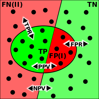
<span class="mw-page-title-main">Evaluation of binary classifiers</span>

The evaluation of binary classifiers compares two methods of assigning a binary attribute, one of which is usually a standard method and the other is being investigated. There are many metrics that can be used to measure the performance of a classifier or predictor; different fields have different preferences for specific metrics due to different goals. For example, in medicine sensitivity and specificity are often used, while in computer science precision and recall are preferred. An important distinction is between metrics that are independent on the prevalence, and metrics that depend on the prevalence – both types are useful, but they have very different properties.

In statistics, Yule's Y, also known as the coefficient of colligation, is a measure of association between two binary variables. The measure was developed by George Udny Yule in 1912, and should not be confused with Yule's coefficient for measuring skewness based on quartiles.

Ordinal data is a categorical, statistical data type where the variables have natural, ordered categories and the distances between the categories are not known. These data exist on an ordinal scale, one of four levels of measurement described by S. S. Stevens in 1946. The ordinal scale is distinguished from the nominal scale by having a ranking. It also differs from the interval scale and ratio scale by not having category widths that represent equal increments of the underlying attribute.

References

↑ Karl Pearson, F.R.S. (1904). Mathematical contributions to the theory of evolution. Dulau and Co.
↑ Ferguson, G. A. (1966). Statistical analysis in psychology and education. New York: McGraw–Hill.
↑ Smith, S. C., & Albaum, G. S. (2004) Fundamentals of marketing research. Sage: Thousand Oaks, CA. p. 631
↑ Blaikie, N. (2003) Analyzing Quantitative Data. Sage: Thousand Oaks, CA. p. 100
↑ Ferguson.^{[ full citation needed ]}
↑ Ferguson, 1966, p. 244
↑ "The Search for Categorical Correlation". 26 December 2019.

External links

This page is based on this Wikipedia article
Text is available under the CC BY-SA 4.0 license; additional terms may apply.
Images, videos and audio are available under their respective licenses.

[1] Karl Pearson, F.R.S. (1904). Mathematical contributions to the theory of evolution. Dulau and Co.

[2] Ferguson, G. A. (1966). Statistical analysis in psychology and education. New York: McGraw–Hill.

[3] Smith, S. C., & Albaum, G. S. (2004) Fundamentals of marketing research. Sage: Thousand Oaks, CA. p. 631

[4] Blaikie, N. (2003) Analyzing Quantitative Data. Sage: Thousand Oaks, CA. p. 100

[5] Ferguson.^{[ full citation needed ]}

[6] Ferguson, 1966, p. 244

[7] "The Search for Categorical Correlation". 26 December 2019.

[1]

[2]

[3]

[4]

[5]

[6]

[7]