Up-and-Down Designs

Last updated

Up-and-down designs (UDDs) are a family of statistical experiment designs used in dose-finding experiments in science, engineering, and medical research. Dose-finding experiments have binary responses: each individual outcome can be described as one of two possible values, such as success vs. failure or toxic vs. non-toxic. Mathematically the binary responses are coded as 1 and 0. The goal of dose-finding experiments is to estimate the strength of treatment (i.e., the "dose") that would trigger the "1" response a pre-specified proportion of the time. This dose can be envisioned as a percentile of the distribution of response thresholds. An example where dose-finding is used is in an experiment to estimate the LD50 of some toxic chemical with respect to mice.

Contents

Simulated experiments from three different UDDs. 0 and 1 responses are marked by o and x, respectively. Top to bottom: the original "simple" UDD that targets the median, a Durham-Flournoy biased-coin UDD targeting approximately the 20.6% percentile, and a k-in-a-row / "transformed" UDD targeting the same percentile. UpAndDownFig1.jpg
Simulated experiments from three different UDDs. 0 and 1 responses are marked by o and x, respectively. Top to bottom: the original "simple" UDD that targets the median, a Durham-Flournoy biased-coin UDD targeting approximately the 20.6% percentile, and a k-in-a-row / "transformed" UDD targeting the same percentile.

Dose-finding designs are sequential and response-adaptive: the dose at a given point in the experiment depends upon previous outcomes, rather than be fixed a priori. Dose-finding designs are generally more efficient for this task than fixed designs, but their properties are harder to analyze, and some require specialized design software. UDDs use a discrete set of doses rather than vary the dose continuously. They are relatively simple to implement, and are also among the best understood dose-finding designs. Despite this simplicity, UDDs generate random walks with intricate properties. [1] The original UDD aimed to find the median threshold by increasing the dose one level after a "0" response, and decreasing it one level after a "1" response. Hence the name "up-and-down". Other UDDs break this symmetry in order to estimate percentiles other than the median, or are able to treat groups of subjects rather than one at a time.

UDDs were developed in the 1940s by several research groups independently. [2] [3] [4] The 1950s and 1960s saw rapid diversification with UDDs targeting percentiles other than the median, and expanding into numerous applied fields. The 1970s to early 1990s saw little UDD methods research, even as the design continued to be used extensively. A revival of UDD research since the 1990s has provided deeper understanding of UDDs and their properties, [5] and new and better estimation methods. [6] [7]

UDDs are still used extensively in the two applications for which they were originally developed: psychophysics where they are used to estimate sensory thresholds and are often known as fixed forced-choice staircase procedures, [8] and explosive sensitivity testing, where the median-targeting UDD is often known as the Bruceton test. UDDs are also very popular in toxicity and anesthesiology research. [9] They are also considered a viable choice for Phase I clinical trials. [10]

Mathematical description

Definition

Let be the sample size of a UDD experiment, and assuming for now that subjects are treated one at a time. Then the doses these subjects receive, denoted as random variables , are chosen from a discrete, finite set of increasing dose levels Furthermore, if , then according to simple constant rules based on recent responses. The next subject must be treated one level up, one level down, or at the same level as the current subject. The responses themselves are denoted hereafter the "1" responses are positive and "0" negative. The repeated application of the same rules (known as dose-transition rules) over a finite set of dose levels, turns into a random walk over . Different dose-transition rules produce different UDD "flavors", such as the three shown in the figure above.

Despite the experiment using only a discrete set of dose levels, the dose-magnitude variable itself, , is assumed to be continuous, and the probability of positive response is assumed to increase continuously with increasing . The goal of dose-finding experiments is to estimate the dose (on a continuous scale) that would trigger positive responses at a pre-specified target rate ; often known as the "target dose". This problem can be also expressed as estimation of the quantile of a cumulative distribution function describing the dose-toxicity curve . The density function associated with is interpretable as the distribution of response thresholds of the population under study.

Transition probability matrix

Given that a subject receives dose , denote the probability that the next subject receives dose , or , as or , respectively. These transition probabilities obey the constraints and the boundary conditions .

Each specific set of UDD rules enables the symbolic calculation of these probabilities, usually as a function of . Assuming that transition probabilities are fixed in time, depending only upon the current allocation and its outcome, i.e., upon and through them upon (and possibly on a set of fixed parameters). The probabilities are then best represented via a tri-diagonal transition probability matrix (TPM) :

Balance point

Usually, UDD dose-transition rules bring the dose down (or at least bar it from escalating) after positive responses, and vice versa. Therefore, UDD random walks have a central tendency: dose assignments tend to meander back and forth around some dose that can be calculated from the transition rules, when those are expressed as a function of . [1] This dose has often been confused with the experiment's formal target , and the two are often identical - but they do not have to be. The target is the dose that the experiment is tasked with estimating, while , known as the "balance point", is approximately where the UDD's random walk revolves around. [11]

Stationary distribution of dose allocations

Since UDD random walks are regular Markov chains, they generate a stationary distribution of dose allocations, , once the effect of the manually-chosen starting dose wears off. This means, long-term visit frequencies to the various doses will approximate a steady state described by . According to Markov chain theory the starting-dose effect wears off rather quickly, at a geometric rate. [12] Numerical studies suggest that it would typically take between and subjects for the effect to wear off nearly completely. [11] is also the asymptotic distribution of cumulative dose allocations.

UDDs' central tendencies ensure that long-term, the most frequently visited dose (i.e., the mode of ) will be one of the two doses closest to the balance point . [1] If is outside the range of allowed doses, then the mode will be on the boundary dose closest to it. Under the original median-finding UDD, the mode will be at the closest dose to in any case. Away from the mode, asymptotic visit frequencies decrease sharply, at a faster-than-geometric rate. Even though a UDD experiment is still a random walk, long excursions away from the region of interest are very unlikely.

Examples of UDD stationary distributions with
M
=
10
{\displaystyle M=10}
. Left: original ("classical") UDD,
x
*
=
5.6
{\displaystyle x^{*}=5.6}
. Right: biased-coin targeting the 30th percentile,
x
*
[?]
3.9.
{\displaystyle x^{*}\approx 3.9.} Pifig.pdf
Examples of UDD stationary distributions with . Left: original ("classical") UDD, . Right: biased-coin targeting the 30th percentile,

Common UDDs

Original ("simple" or "classical") UDD

The original "simple" or "classical" UDD moves the dose up one level upon a negative response, and vice versa. Therefore, the transition probabilities are

We use the original UDD as an example for calculating the balance point . The design's 'up', 'down' functions are We equate them to find :

The "classical" UDD is designed to find the median threshold. This is a case where

The "classical" UDD can be seen as a special case of each of the more versatile designs described below.

Durham and Flournoy's biased coin design

This UDD shifts the balance point, by adding the option of treating the next subject at the same dose rather than move only up or down. Whether to stay is determined by a random toss of a metaphoric "coin" with probability This biased-coin design (BCD) has two "flavors", one for and one for whose rules are shown below:

The heads probability can take any value in. The balance point is

The BCD balance point can made identical to a target rate by setting the heads probability to . For example, for set . Setting makes this design identical to the classical UDD, and inverting the rules by imposing the coin toss upon positive rather than negative outcomes, produces above-median balance points. Versions with two coins, one for each outcome, have also been published, but they do not seem to offer an advantage over the simpler single-coin BCD.

Group (cohort) UDDs

Some dose-finding experiments, such as phase I trials, require a waiting period of weeks before determining each individual outcome. It may preferable then, to be able treat several subjects at once or in rapid succession. With group UDDs, the transition rules apply rules to cohorts of fixed size rather than to individuals. becomes the dose given to cohort , and is the number of positive responses in the -th cohort, rather than a binary outcome. Given that the -th cohort is treated at on the interior of the -th cohort is assigned to

follow a binomial distribution conditional on , with parameters and. The up and down probabilities are the binomial distribution's tails, and the stay probability its center (it is zero if ). A specific choice of parameters can be abbreviated as GUD

Nominally, group UDDs generate -order random walks, since the most recent observations are needed to determine the next allocation. However, with cohorts viewed as single mathematical entities, these designs generate a first-order random walk having a tri-diagonal TPM as above. Some relevant group UDD subfamilies:

With would be associated with and , respectively. The mirror-image family GUD has its balance points at one minus these probabilities.

For general group UDDs, the balance point can be calculated only numerically, by finding the dose with toxicity rate such that

Any numerical root-finding algorithm, e.g., Newton–Raphson, can be used to solve for . [13]

-in-a-row (or "transformed" or "geometric") UDD

This is the most commonly used non-median UDD. It was introduced by Wetherill in 1963, [14] and proliferated by him and colleagues shortly thereafter to psychophysics, [15] where it remains one of the standard methods to find sensory thresholds. [8] Wetherill called it "transformed" UDD; Gezmu who was the first to analyze its random-walk properties, called it "Geometric" UDD in the 1990s; [16] and in the 2000s the more straightforward name "-in-a-row" UDD was adopted. [11] The design's rules are deceptively simple:

Every dose escalation requires non-toxicities observed on consecutive data points, all at the current dose, while de-escalation only requires a single toxicity. It closely resembles GUD described above, and indeed shares the same balance point. The difference is that -in-a-row can bail out of a dose level upon the first toxicity, whereas its group UDD sibling might treat the entire cohort at once, and therefore might see more than one toxicity before descending.

The method used in sensory studies is actually the mirror-image of the one defined above, with successive responses required for a de-escalation and only one non-response for escalation, yielding for . [17]

-in-a-row generates a -th order random walk because knowledge of the last responses might be needed. It can be represented as a first-order chain with states, or as a Markov chain with levels, each having internal states labeled to The internal state serves as a counter of the number of immediately recent consecutive non-toxicities observed at the current dose. This description is closer to the physical dose-allocation process, because subjects at different internal states of the level , are all assigned the same dose . Either way, the TPM is (or more precisely, , because the internal counter is meaningless at the highest dose) - and it is not tridiagonal.

Here is the expanded -in-a-row TPM with and , using the abbreviation Each level's internal states are adjacent to each other.

-in-a-row is often considered for clinical trials targeting a low-toxicity dose. In this case, the balance point and the target are not identical; rather, is chosen to aim close to the target rate, e.g., for studies targeting the 30th percentile, and for studies targeting the 20th percentile.

Estimating the target dose

Example for reversal-averaging estimation of a psychophysics experiment. Reversal points are circled, and the first reversal was excluded from the average. The design is a two-stage, with the second (and main) stage
k
{\displaystyle k}
-in-a-row targeting the 70.7% percentile. The first stage (until the first reversal) uses the "classical" UDD, a commonly-employed scheme to speed up the arrival to the region of interest. Staircase Transformed Up Down English.png
Example for reversal-averaging estimation of a psychophysics experiment. Reversal points are circled, and the first reversal was excluded from the average. The design is a two-stage, with the second (and main) stage -in-a-row targeting the 70.7% percentile. The first stage (until the first reversal) uses the "classical" UDD, a commonly-employed scheme to speed up the arrival to the region of interest.

Unlike other design approaches, UDDs do not have a specific estimation method "bundled in" with the design as a default choice. Historically, the more common choice has been some weighted average of the doses administered, usually excluding the first few doses to mitigate the starting-point bias. This approach antedates deeper understanding of UDDs' Markov properties, but its success in numerical evaluations relies upon the eventual sampling from , since the latter is centered roughly around [5]

The single most popular among these averaging estimators was introduced by Wetherill et al. in 1966, and only includes reversal points (points where the outcome switches from 0 to 1 or vice versa) in the average. [18] In recent years, the limitations of averaging estimators have come to light, in particular the many sources of bias that are very difficult to mitigate. Reversal estimators suffer from both multiple biases (although there is some inadvertent cancelling out of biases), and increased variance due to using a subsample of doses. However, the knowledge about averaging-estimator limitations has yet to disseminate outside the methodological literature and affect actual practice. [5]

By contrast, regression estimators attempt to approximate the curve describing the dose-response relationship, in particular around the target percentile. The raw data for the regression are the doses on the horizontal axis, and the observed toxicity frequencies,

on the vertical axis. The target estimate is the abscissa of the point where the fitted curve crosses

Probit regression has been used for many decades to estimate UDD targets, although far less commonly than the reversal-averaging estimator. In 2002, Stylianou and Flournoy introduced an interpolated version of isotonic regression (IR) to estimate UDD targets and other dose-response data. [6] More recently, a modification called "centered isotonic regression" (CIR) was developed by Oron and Flournoy, promising substantially better estimation performance than ordinary isotonic regression in most cases, and also offering the first viable interval estimator for isotonic regression in general. [7] Isotonic regression estimators appear to be the most compatible with UDDs, because both approaches are nonparametric and relatively robust. [5] The publicly available R package "cir" implements both CIR and IR for dose-finding and other applications. [19]

Related Research Articles

<span class="mw-page-title-main">Cauchy distribution</span> Probability distribution

The Cauchy distribution, named after Augustin Cauchy, is a continuous probability distribution. It is also known, especially among physicists, as the Lorentz distribution, Cauchy–Lorentz distribution, Lorentz(ian) function, or Breit–Wigner distribution. The Cauchy distribution is the distribution of the x-intercept of a ray issuing from with a uniformly distributed angle. It is also the distribution of the ratio of two independent normally distributed random variables with mean zero.

<span class="mw-page-title-main">Negative binomial distribution</span> Probability distribution

In probability theory and statistics, the negative binomial distribution is a discrete probability distribution that models the number of failures in a sequence of independent and identically distributed Bernoulli trials before a specified (non-random) number of successes occurs. For example, we can define rolling a 6 on a dice as a success, and rolling any other number as a failure, and ask how many failure rolls will occur before we see the third success. In such a case, the probability distribution of the number of failures that appear will be a negative binomial distribution.

In statistics, the Gauss–Markov theorem states that the ordinary least squares (OLS) estimator has the lowest sampling variance within the class of linear unbiased estimators, if the errors in the linear regression model are uncorrelated, have equal variances and expectation value of zero. The errors do not need to be normal, nor do they need to be independent and identically distributed. The requirement that the estimator be unbiased cannot be dropped, since biased estimators exist with lower variance. See, for example, the James–Stein estimator, ridge regression, or simply any degenerate estimator.

<span class="mw-page-title-main">Gamma distribution</span> Probability distribution

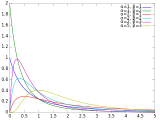
In probability theory and statistics, the gamma distribution is a two-parameter family of continuous probability distributions. The exponential distribution, Erlang distribution, and chi-squared distribution are special cases of the gamma distribution. There are two equivalent parameterizations in common use:

  1. With a shape parameter and a scale parameter .
  2. With a shape parameter and an inverse scale parameter , called a rate parameter.
<span class="mw-page-title-main">Kriging</span> Method of interpolation

In statistics, originally in geostatistics, kriging or Kriging, also known as Gaussian process regression, is a method of interpolation based on Gaussian process governed by prior covariances. Under suitable assumptions of the prior, kriging gives the best linear unbiased prediction (BLUP) at unsampled locations. Interpolating methods based on other criteria such as smoothness may not yield the BLUP. The method is widely used in the domain of spatial analysis and computer experiments. The technique is also known as Wiener–Kolmogorov prediction, after Norbert Wiener and Andrey Kolmogorov.

In statistics, a generalized linear model (GLM) is a flexible generalization of ordinary linear regression. The GLM generalizes linear regression by allowing the linear model to be related to the response variable via a link function and by allowing the magnitude of the variance of each measurement to be a function of its predicted value.

The Newmark-beta method is a method of numerical integration used to solve certain differential equations. It is widely used in numerical evaluation of the dynamic response of structures and solids such as in finite element analysis to model dynamic systems. The method is named after Nathan M. Newmark, former Professor of Civil Engineering at the University of Illinois at Urbana–Champaign, who developed it in 1959 for use in structural dynamics. The semi-discretized structural equation is a second order ordinary differential equation system,

<span class="mw-page-title-main">Statistical learning theory</span> Framework for machine learning

Statistical learning theory is a framework for machine learning drawing from the fields of statistics and functional analysis. Statistical learning theory deals with the statistical inference problem of finding a predictive function based on data. Statistical learning theory has led to successful applications in fields such as computer vision, speech recognition, and bioinformatics.

<span class="mw-page-title-main">Laplace distribution</span> Probability distribution

In probability theory and statistics, the Laplace distribution is a continuous probability distribution named after Pierre-Simon Laplace. It is also sometimes called the double exponential distribution, because it can be thought of as two exponential distributions spliced together along the abscissa, although the term is also sometimes used to refer to the Gumbel distribution. The difference between two independent identically distributed exponential random variables is governed by a Laplace distribution, as is a Brownian motion evaluated at an exponentially distributed random time. Increments of Laplace motion or a variance gamma process evaluated over the time scale also have a Laplace distribution.

In probability theory and statistics, the generalized extreme value (GEV) distribution is a family of continuous probability distributions developed within extreme value theory to combine the Gumbel, Fréchet and Weibull families also known as type I, II and III extreme value distributions. By the extreme value theorem the GEV distribution is the only possible limit distribution of properly normalized maxima of a sequence of independent and identically distributed random variables. Note that a limit distribution needs to exist, which requires regularity conditions on the tail of the distribution. Despite this, the GEV distribution is often used as an approximation to model the maxima of long (finite) sequences of random variables.

<span class="mw-page-title-main">Inverse-gamma distribution</span> Two-parameter family of continuous probability distributions

In probability theory and statistics, the inverse gamma distribution is a two-parameter family of continuous probability distributions on the positive real line, which is the distribution of the reciprocal of a variable distributed according to the gamma distribution.

<span class="mw-page-title-main">Kumaraswamy distribution</span>

In probability and statistics, the Kumaraswamy's double bounded distribution is a family of continuous probability distributions defined on the interval (0,1). It is similar to the Beta distribution, but much simpler to use especially in simulation studies since its probability density function, cumulative distribution function and quantile functions can be expressed in closed form. This distribution was originally proposed by Poondi Kumaraswamy for variables that are lower and upper bounded with a zero-inflation. This was extended to inflations at both extremes [0,1] in later work with S. G. Fletcher.

<span class="mw-page-title-main">Isotonic regression</span> Type of numerical analysis

In statistics and numerical analysis, isotonic regression or monotonic regression is the technique of fitting a free-form line to a sequence of observations such that the fitted line is non-decreasing everywhere, and lies as close to the observations as possible.

<span class="mw-page-title-main">Beta prime distribution</span> Probability distribution

In probability theory and statistics, the beta prime distribution is an absolutely continuous probability distribution. If has a beta distribution, then the odds has a beta prime distribution.

In statistics, M-estimators are a broad class of extremum estimators for which the objective function is a sample average. Both non-linear least squares and maximum likelihood estimation are special cases of M-estimators. The definition of M-estimators was motivated by robust statistics, which contributed new types of M-estimators. However, M-estimators are not inherently robust, as is clear from the fact that they include maximum likelihood estimators, which are in general not robust. The statistical procedure of evaluating an M-estimator on a data set is called M-estimation.

The cross-entropy (CE) method is a Monte Carlo method for importance sampling and optimization. It is applicable to both combinatorial and continuous problems, with either a static or noisy objective.

In statistics, explained variation measures the proportion to which a mathematical model accounts for the variation (dispersion) of a given data set. Often, variation is quantified as variance; then, the more specific term explained variance can be used.

<span class="mw-page-title-main">Log-logistic distribution</span>

In probability and statistics, the log-logistic distribution is a continuous probability distribution for a non-negative random variable. It is used in survival analysis as a parametric model for events whose rate increases initially and decreases later, as, for example, mortality rate from cancer following diagnosis or treatment. It has also been used in hydrology to model stream flow and precipitation, in economics as a simple model of the distribution of wealth or income, and in networking to model the transmission times of data considering both the network and the software.

The Vanna–Volga method is a mathematical tool used in finance. It is a technique for pricing first-generation exotic options in foreign exchange market (FX) derivatives.

Inverse probability weighting is a statistical technique for calculating statistics standardized to a pseudo-population different from that in which the data was collected. Study designs with a disparate sampling population and population of target inference are common in application. There may be prohibitive factors barring researchers from directly sampling from the target population such as cost, time, or ethical concerns. A solution to this problem is to use an alternate design strategy, e.g. stratified sampling. Weighting, when correctly applied, can potentially improve the efficiency and reduce the bias of unweighted estimators.

References

  1. 1 2 3 Durham, SD; Flournoy, N. "Up-and-down designs. I. Stationary treatment distributions.". In Flournoy, N; Rosenberger, WF (eds.). IMS Lecture Notes Monograph Series. Vol. 25: Adaptive Designs. pp. 139–157.
  2. Dixon, WJ; Mood, AM (1948). "A method for obtaining and analyzing sensitivity data". Journal of the American Statistical Association. 43 (241): 109–126. doi:10.1080/01621459.1948.10483254.
  3. von Békésy, G (1947). "A new audiometer". Acta Oto-Laryngologica. 35 (5–6): 411–422. doi:10.3109/00016484709123756.
  4. Anderson, TW; McCarthy, PJ; Tukey, JW (1946). 'Staircase' method of sensitivity testing (Technical report). Naval Ordnance Report. 65-46.
  5. 1 2 3 4 Flournoy, N; Oron, AP. "Up-and-Down Designs for Dose-Finding". In Dean, A (ed.). Handbook of Design and Analysis of Experiments. CRC Press. pp. 858–894.
  6. 1 2 Stylianou, MP; Flournoy, N (2002). "Dose finding using the biased coin up-and-down design and isotonic regression". Biometrics. 58 (1): 171–177. doi:10.1111/j.0006-341x.2002.00171.x. PMID   11890313. S2CID   8743090.
  7. 1 2 Oron, AP; Flournoy, N (2017). "Centered Isotonic Regression: Point and Interval Estimation for Dose-Response Studies". Statistics in Biopharmaceutical Research. 9 (3): 258–267. arXiv: 1701.05964 . doi:10.1080/19466315.2017.1286256. S2CID   88521189.
  8. 1 2 Leek, MR (2001). "Adaptive procedures in psychophysical research". Perception and Psychophysics. 63 (8): 1279–1292. doi: 10.3758/bf03194543 . PMID   11800457.
  9. Pace, NL; Stylianou, MP (2007). "Advances in and Limitations of Up-and-down Methodology: A Precis of Clinical Use, Study Design, and Dose Estimation in Anesthesia Research". Anesthesiology. 107 (1): 144–152. doi: 10.1097/01.anes.0000267514.42592.2a . PMID   17585226.
  10. Oron, AP; Hoff, PD (2013). "Small-Sample Behavior of Novel Phase I Cancer Trial Designs". Clinical Trials. 10 (1): 63–80. arXiv: 1202.4962 . doi:10.1177/1740774512469311. PMID   23345304. S2CID   5667047.
  11. 1 2 3 Oron, AP; Hoff, PD (2009). "The k-in-a-row up-and-down design, revisited". Statistics in Medicine. 28 (13): 1805–1820. doi:10.1002/sim.3590. PMID   19378270. S2CID   25904900.
  12. Diaconis, P; Stroock, D (1991). "Geometric bounds for eigenvalues of Markov chain". The Annals of Applied Probability. 1: 36–61. doi: 10.1214/aoap/1177005980 .
  13. Gezmu, M; Flournoy, N (2006). "Group up-and-down designs for dose-finding". Journal of Statistical Planning and Inference. 136 (6): 1749–1764. doi:10.1016/j.jspi.2005.08.002.
  14. Wetherill, GB; Levitt, H (1963). "Sequential estimation of quantal response curves". Journal of the Royal Statistical Society, Series B. 25: 1–48. doi:10.1111/j.2517-6161.1963.tb00481.x.
  15. Wetherill, GB (1965). "Sequential estimation of points on a Psychometric Function". British Journal of Mathematical and Statistical Psychology. 18: 1–10. doi:10.1111/j.2044-8317.1965.tb00689.x. PMID   14324842.
  16. Gezmu, Misrak (1996). The Geometric Up-and-Down Design for Allocating Dosage Levels (PhD). American University.
  17. Garcia-Perez, MA (1998). "Forced-choice staircases with fixed step sizes: asymptotic and small-sample properties". Vision Research. 38 (12): 1861–81. doi: 10.1016/s0042-6989(97)00340-4 . PMID   9797963.
  18. Wetherill, GB; Chen, H; Vasudeva, RB (1966). "Sequential estimation of quantal response curves: a new method of estimation". Biometrika. 53 (3–4): 439–454. doi:10.1093/biomet/53.3-4.439.
  19. Oron, Assaf. "Package 'cir'". CRAN. R Foundation for Statistical Computing. Retrieved 26 December 2020.