
In statistics, an estimator is a rule for calculating an estimate of a given quantity based on observed data: thus the rule, the quantity of interest and its result are distinguished. For example, the sample mean is a commonly used estimator of the population mean.

Statistical inference is the process of using data analysis to infer properties of an underlying distribution of probability. Inferential statistical analysis infers properties of a population, for example by testing hypotheses and deriving estimates. It is assumed that the observed data set is sampled from a larger population.
The following outline is provided as an overview of and topical guide to statistics:
The likelihood function is the joint probability mass of observed data viewed as a function of the parameters of a statistical model. Intuitively, the likelihood function is the probability of observing data assuming is the actual parameter.
In statistics, maximum likelihood estimation (MLE) is a method of estimating the parameters of an assumed probability distribution, given some observed data. This is achieved by maximizing a likelihood function so that, under the assumed statistical model, the observed data is most probable. The point in the parameter space that maximizes the likelihood function is called the maximum likelihood estimate. The logic of maximum likelihood is both intuitive and flexible, and as such the method has become a dominant means of statistical inference.
In statistics, interval estimation is the use of sample data to estimate an interval of possible values of a parameter of interest. This is in contrast to point estimation, which gives a single value.
In statistics, completeness is a property of a statistic in relation to a parameterised model for a set of observed data.
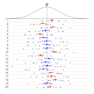
Informally, in frequentist statistics, a confidence interval (CI) is an interval which is expected to typically contain the parameter being estimated. More specifically, given a confidence level , a CI is a random interval which contains the parameter being estimated % of the time. The confidence level, degree of confidence or confidence coefficient represents the long-run proportion of CIs that theoretically contain the true value of the parameter; this is tantamount to the nominal coverage probability. For example, out of all intervals computed at the 95% level, 95% of them should contain the parameter's true value.
In statistical inference, specifically predictive inference, a prediction interval is an estimate of an interval in which a future observation will fall, with a certain probability, given what has already been observed. Prediction intervals are often used in regression analysis.

In statistics, a consistent estimator or asymptotically consistent estimator is an estimator—a rule for computing estimates of a parameter θ0—having the property that as the number of data points used increases indefinitely, the resulting sequence of estimates converges in probability to θ0. This means that the distributions of the estimates become more and more concentrated near the true value of the parameter being estimated, so that the probability of the estimator being arbitrarily close to θ0 converges to one.
Estimation theory is a branch of statistics that deals with estimating the values of parameters based on measured empirical data that has a random component. The parameters describe an underlying physical setting in such a way that their value affects the distribution of the measured data. An estimator attempts to approximate the unknown parameters using the measurements. In estimation theory, two approaches are generally considered:
Bootstrapping is any test or metric that uses random sampling with replacement, and falls under the broader class of resampling methods. Bootstrapping assigns measures of accuracy to sample estimates. This technique allows estimation of the sampling distribution of almost any statistic using random sampling methods.
In estimation theory and decision theory, a Bayes estimator or a Bayes action is an estimator or decision rule that minimizes the posterior expected value of a loss function. Equivalently, it maximizes the posterior expectation of a utility function. An alternative way of formulating an estimator within Bayesian statistics is maximum a posteriori estimation.
In statistics, shrinkage is the reduction in the effects of sampling variation. In regression analysis, a fitted relationship appears to perform less well on a new data set than on the data set used for fitting. In particular the value of the coefficient of determination 'shrinks'. This idea is complementary to overfitting and, separately, to the standard adjustment made in the coefficient of determination to compensate for the subjunctive effects of further sampling, like controlling for the potential of new explanatory terms improving the model by chance: that is, the adjustment formula itself provides "shrinkage." But the adjustment formula yields an artificial shrinkage.
In statistics, the bias of an estimator is the difference between this estimator's expected value and the true value of the parameter being estimated. An estimator or decision rule with zero bias is called unbiased. In statistics, "bias" is an objective property of an estimator. Bias is a distinct concept from consistency: consistent estimators converge in probability to the true value of the parameter, but may be biased or unbiased; see bias versus consistency for more.
In statistics, Fisher consistency, named after Ronald Fisher, is a desirable property of an estimator asserting that if the estimator were calculated using the entire population rather than a sample, the true value of the estimated parameter would be obtained.

In statistics, maximum spacing estimation (MSE or MSP), or maximum product of spacing estimation (MPS), is a method for estimating the parameters of a univariate statistical model. The method requires maximization of the geometric mean of spacings in the data, which are the differences between the values of the cumulative distribution function at neighbouring data points.
In statistics, efficiency is a measure of quality of an estimator, of an experimental design, or of a hypothesis testing procedure. Essentially, a more efficient estimator needs fewer input data or observations than a less efficient one to achieve the Cramér–Rao bound. An efficient estimator is characterized by having the smallest possible variance, indicating that there is a small deviance between the estimated value and the "true" value in the L2 norm sense.
In statistical inference, the concept of a confidence distribution (CD) has often been loosely referred to as a distribution function on the parameter space that can represent confidence intervals of all levels for a parameter of interest. Historically, it has typically been constructed by inverting the upper limits of lower sided confidence intervals of all levels, and it was also commonly associated with a fiducial interpretation, although it is a purely frequentist concept. A confidence distribution is NOT a probability distribution function of the parameter of interest, but may still be a function useful for making inferences.
In Bayesian inference, the Bernstein–von Mises theorem provides the basis for using Bayesian credible sets for confidence statements in parametric models. It states that under some conditions, a posterior distribution converges in the limit of infinite data to a multivariate normal distribution centered at the maximum likelihood estimator with covariance matrix given by , where is the true population parameter and is the Fisher information matrix at the true population parameter value:
