In statistics, an estimator is a rule for calculating an estimate of a given quantity based on observed data: thus the rule, the quantity of interest and its result are distinguished. For example, the sample mean is a commonly used estimator of the population mean.
In statistics, a location parameter of a probability distribution is a scalar- or vector-valued parameter , which determines the "location" or shift of the distribution. In the literature of location parameter estimation, the probability distributions with such parameter are found to be formally defined in one of the following equivalent ways:
In statistics, maximum likelihood estimation (MLE) is a method of estimating the parameters of an assumed probability distribution, given some observed data. This is achieved by maximizing a likelihood function so that, under the assumed statistical model, the observed data is most probable. The point in the parameter space that maximizes the likelihood function is called the maximum likelihood estimate. The logic of maximum likelihood is both intuitive and flexible, and as such the method has become a dominant means of statistical inference.
In statistics, the mean squared error (MSE) or mean squared deviation (MSD) of an estimator measures the average of the squares of the errors—that is, the average squared difference between the estimated values and the actual value. MSE is a risk function, corresponding to the expected value of the squared error loss. The fact that MSE is almost always strictly positive is because of randomness or because the estimator does not account for information that could produce a more accurate estimate. In machine learning, specifically empirical risk minimization, MSE may refer to the empirical risk, as an estimate of the true MSE.
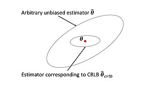
In estimation theory and statistics, the Cramér–Rao bound (CRB) relates to estimation of a deterministic parameter. The result is named in honor of Harald Cramér and C. R. Rao, but has also been derived independently by Maurice Fréchet, Georges Darmois, and by Alexander Aitken and Harold Silverstone. It is also known as Fréchet-Cramér–Rao or Fréchet-Darmois-Cramér-Rao lower bound. It states that the precision of any unbiased estimator is at most the Fisher information; or (equivalently) the reciprocal of the Fisher information is a lower bound on its variance.
In mathematical statistics, the Fisher information is a way of measuring the amount of information that an observable random variable X carries about an unknown parameter θ of a distribution that models X. Formally, it is the variance of the score, or the expected value of the observed information.
Directional statistics is the subdiscipline of statistics that deals with directions, axes or rotations in Rn. More generally, directional statistics deals with observations on compact Riemannian manifolds including the Stiefel manifold.
In Bayesian statistics, a maximum a posteriori probability (MAP) estimate is an estimate of an unknown quantity, that equals the mode of the posterior distribution. The MAP can be used to obtain a point estimate of an unobserved quantity on the basis of empirical data. It is closely related to the method of maximum likelihood (ML) estimation, but employs an augmented optimization objective which incorporates a prior distribution over the quantity one wants to estimate. MAP estimation can therefore be seen as a regularization of maximum likelihood estimation.

In probability theory, the Rice distribution or Rician distribution is the probability distribution of the magnitude of a circularly-symmetric bivariate normal random variable, possibly with non-zero mean (noncentral). It was named after Stephen O. Rice (1907–1986).
In Bayesian statistics, the Jeffreys prior is a non-informative prior distribution for a parameter space. Named after Sir Harold Jeffreys, its density function is proportional to the square root of the determinant of the Fisher information matrix:
In statistics, the Bayesian information criterion (BIC) or Schwarz information criterion is a criterion for model selection among a finite set of models; models with lower BIC are generally preferred. It is based, in part, on the likelihood function and it is closely related to the Akaike information criterion (AIC).
The James–Stein estimator is a biased estimator of the mean, , of (possibly) correlated Gaussian distributed random variables with unknown means .
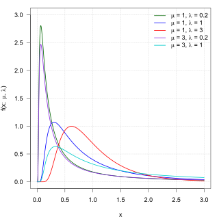
In probability theory, the inverse Gaussian distribution is a two-parameter family of continuous probability distributions with support on (0,∞).
In statistics, the bias of an estimator is the difference between this estimator's expected value and the true value of the parameter being estimated. An estimator or decision rule with zero bias is called unbiased. In statistics, "bias" is an objective property of an estimator. Bias is a distinct concept from consistency: consistent estimators converge in probability to the true value of the parameter, but may be biased or unbiased.

In probability theory and statistics, the half-normal distribution is a special case of the folded normal distribution.
In statistical decision theory, where we are faced with the problem of estimating a deterministic parameter (vector) from observations an estimator is called minimax if its maximal risk is minimal among all estimators of . In a sense this means that is an estimator which performs best in the worst possible case allowed in the problem.

In probability theory and directional statistics, a wrapped normal distribution is a wrapped probability distribution that results from the "wrapping" of the normal distribution around the unit circle. It finds application in the theory of Brownian motion and is a solution to the heat equation for periodic boundary conditions. It is closely approximated by the von Mises distribution, which, due to its mathematical simplicity and tractability, is the most commonly used distribution in directional statistics.
In statistics, efficiency is a measure of quality of an estimator, of an experimental design, or of a hypothesis testing procedure. Essentially, a more efficient estimator needs fewer input data or observations than a less efficient one to achieve the Cramér–Rao bound. An efficient estimator is characterized by having the smallest possible variance, indicating that there is a small deviance between the estimated value and the "true" value in the L2 norm sense.
In statistical inference, the concept of a confidence distribution (CD) has often been loosely referred to as a distribution function on the parameter space that can represent confidence intervals of all levels for a parameter of interest. Historically, it has typically been constructed by inverting the upper limits of lower sided confidence intervals of all levels, and it was also commonly associated with a fiducial interpretation, although it is a purely frequentist concept. A confidence distribution is NOT a probability distribution function of the parameter of interest, but may still be a function useful for making inferences.
Bayesian hierarchical modelling is a statistical model written in multiple levels that estimates the parameters of the posterior distribution using the Bayesian method. The sub-models combine to form the hierarchical model, and Bayes' theorem is used to integrate them with the observed data and account for all the uncertainty that is present. The result of this integration is the posterior distribution, also known as the updated probability estimate, as additional evidence on the prior distribution is acquired.


