Partial derivative

In mathematics, a partial derivative of a function of several variables is its derivative with respect to one of those variables, with the others held constant (as opposed to the total derivative, in which all variables are allowed to vary). Partial derivatives are used in vector calculus and differential geometry.

The partial derivative of a function ${\displaystyle f(x,y,\dots )}$ with respect to the variable ${\displaystyle x}$ is variously denoted by

${\displaystyle f_{x}}$, ${\displaystyle f'_{x}}$, ${\displaystyle \partial _{x}f}$, ${\displaystyle \ D_{x}f}$, ${\displaystyle D_{1}f}$, ${\displaystyle {\frac {\partial }{\partial x}}f}$, or ${\displaystyle {\frac {\partial f}{\partial x}}}$.

It can be thought of as the rate of change of the function in the ${\displaystyle x}$-direction.

Sometimes, for ${\displaystyle z=f(x,y,\ldots )}$, the partial derivative of ${\displaystyle z}$ with respect to ${\displaystyle x}$ is denoted as ${\displaystyle {\tfrac {\partial z}{\partial x}}.}$ Since a partial derivative generally has the same arguments as the original function, its functional dependence is sometimes explicitly signified by the notation, such as in:

$${\displaystyle f'_{x}(x,y,\ldots ),{\frac {\partial f}{\partial x}}(x,y,\ldots ).}$$

The symbol used to denote partial derivatives is ∂. One of the first known uses of this symbol in mathematics is by Marquis de Condorcet from 1770, ^[1] who used it for partial differences. The modern partial derivative notation was created by Adrien-Marie Legendre (1786), although he later abandoned it; Carl Gustav Jacob Jacobi reintroduced the symbol in 1841. ^[2]

Definition

Like ordinary derivatives, the partial derivative is defined as a limit. Let U be an open subset of ${\displaystyle \mathbb {R} ^{n}}$ and ${\displaystyle f:U\to \mathbb {R} }$ a function. The partial derivative of f at the point ${\displaystyle \mathbf {a} =(a_{1},\ldots ,a_{n})\in U}$ with respect to the i-th variable x_i is defined as

$${\displaystyle {\begin{aligned}{\frac {\partial }{\partial x_{i}}}f(\mathbf {a} )&=\lim _{h\to 0}{\frac {f(a_{1},\ldots ,a_{i-1},a_{i}+h,a_{i+1}\,\ldots ,a_{n})\ -f(a_{1},\ldots ,a_{i},\dots ,a_{n})}{h}}\\&=\lim _{h\to 0}{\frac {f(\mathbf {a} +h\mathbf {e_{i}} )-f(\mathbf {a} )}{h}}\,.\end{aligned}}}$$

Where ${\displaystyle \mathbf {e_{i}} }$ is the unit vector of i-th variable x_i. Even if all partial derivatives ${\displaystyle \partial f/\partial x_{i}(a)}$ exist at a given point a, the function need not be continuous there. However, if all partial derivatives exist in a neighborhood of a and are continuous there, then f is totally differentiable in that neighborhood and the total derivative is continuous. In this case, it is said that f is a C¹ function. This can be used to generalize for vector valued functions, ${\displaystyle f:U\to \mathbb {R} ^{m}}$, by carefully using a componentwise argument.

The partial derivative ${\textstyle {\frac {\partial f}{\partial x}}}$ can be seen as another function defined on U and can again be partially differentiated. If the direction of derivative is not repeated, it is called a mixed partial derivative. If all mixed second order partial derivatives are continuous at a point (or on a set), f is termed a C² function at that point (or on that set); in this case, the partial derivatives can be exchanged by Clairaut's theorem:

$${\displaystyle {\frac {\partial ^{2}f}{\partial x_{i}\partial x_{j}}}={\frac {\partial ^{2}f}{\partial x_{j}\partial x_{i}}}.}$$

Notation

Further information: ∂

For the following examples, let f be a function in x, y, and z.

First-order partial derivatives:

$${\displaystyle {\frac {\partial f}{\partial x}}=f'_{x}=\partial _{x}f.}$$

Second-order partial derivatives:

$${\displaystyle {\frac {\partial ^{2}f}{\partial x^{2}}}=f''_{xx}=\partial _{xx}f=\partial _{x}^{2}f.}$$

Second-order mixed derivatives:

$${\displaystyle {\frac {\partial ^{2}f}{\partial y\,\partial x}}={\frac {\partial }{\partial y}}\left({\frac {\partial f}{\partial x}}\right)=(f'_{x})'_{y}=f''_{xy}=\partial _{yx}f=\partial _{y}\partial _{x}f.}$$

Higher-order partial and mixed derivatives:

$${\displaystyle {\frac {\partial ^{i+j+k}f}{\partial x^{i}\partial y^{j}\partial z^{k}}}=f^{(i,j,k)}=\partial _{x}^{i}\partial _{y}^{j}\partial _{z}^{k}f.}$$

When dealing with functions of multiple variables, some of these variables may be related to each other, thus it may be necessary to specify explicitly which variables are being held constant to avoid ambiguity. In fields such as statistical mechanics, the partial derivative of f with respect to x, holding y and z constant, is often expressed as

$${\displaystyle \left({\frac {\partial f}{\partial x}}\right)_{y,z}.}$$

Conventionally, for clarity and simplicity of notation, the partial derivative function and the value of the function at a specific point are conflated by including the function arguments when the partial derivative symbol (Leibniz notation) is used. Thus, an expression like

$${\displaystyle {\frac {\partial f(x,y,z)}{\partial x}}}$$

is used for the function, while

$${\displaystyle {\frac {\partial f(u,v,w)}{\partial u}}}$$

might be used for the value of the function at the point ${\displaystyle (x,y,z)=(u,v,w)}$. However, this convention breaks down when we want to evaluate the partial derivative at a point like ${\displaystyle (x,y,z)=(17,u+v,v^{2})}$. In such a case, evaluation of the function must be expressed in an unwieldy manner as

$${\displaystyle {\frac {\partial f(x,y,z)}{\partial x}}(17,u+v,v^{2})}$$

or

$${\displaystyle \left.{\frac {\partial f(x,y,z)}{\partial x}}\right|_{(x,y,z)=(17,u+v,v^{2})}}$$

in order to use the Leibniz notation. Thus, in these cases, it may be preferable to use the Euler differential operator notation with ${\displaystyle D_{i}}$ as the partial derivative symbol with respect to the i-th variable. For instance, one would write ${\displaystyle D_{1}f(17,u+v,v^{2})}$ for the example described above, while the expression ${\displaystyle D_{1}f}$ represents the partial derivative function with respect to the first variable. ^[3]

For higher order partial derivatives, the partial derivative (function) of ${\displaystyle D_{i}f}$ with respect to the j-th variable is denoted ${\displaystyle D_{j}(D_{i}f)=D_{i,j}f}$. That is, ${\displaystyle D_{j}\circ D_{i}=D_{i,j}}$, so that the variables are listed in the order in which the derivatives are taken, and thus, in reverse order of how the composition of operators is usually notated. Of course, Clairaut's theorem implies that ${\displaystyle D_{i,j}=D_{j,i}}$ as long as comparatively mild regularity conditions on f are satisfied.

Gradient

Main article: Gradient

An important example of a function of several variables is the case of a scalar-valued function ${\displaystyle f(x_{1},\ldots ,x_{n})}$ on a domain in Euclidean space ${\displaystyle \mathbb {R} ^{n}}$ (e.g., on ${\displaystyle \mathbb {R} ^{2}}$ or ${\displaystyle \mathbb {R} ^{3}}$). In this case f has a partial derivative ${\displaystyle \partial f/\partial x_{j}}$ with respect to each variable x_j. At the point a, these partial derivatives define the vector

$${\displaystyle \nabla f(a)=\left({\frac {\partial f}{\partial x_{1}}}(a),\ldots ,{\frac {\partial f}{\partial x_{n}}}(a)\right).}$$

This vector is called the gradient of f at a. If f is differentiable at every point in some domain, then the gradient is a vector-valued function ∇f which takes the point a to the vector ∇f(a). Consequently, the gradient produces a vector field.

A common abuse of notation is to define the del operator (∇) as follows in three-dimensional Euclidean space ${\displaystyle \mathbb {R} ^{3}}$ with unit vectors ${\displaystyle {\hat {\mathbf {i} }},{\hat {\mathbf {j} }},{\hat {\mathbf {k} }}}$:

$${\displaystyle \nabla =\left[{\frac {\partial }{\partial x}}\right]{\hat {\mathbf {i} }}+\left[{\frac {\partial }{\partial y}}\right]{\hat {\mathbf {j} }}+\left[{\frac {\partial }{\partial z}}\right]{\hat {\mathbf {k} }}}$$

Or, more generally, for n-dimensional Euclidean space ${\displaystyle \mathbb {R} ^{n}}$ with coordinates ${\displaystyle x_{1},\ldots ,x_{n}}$ and unit vectors ${\displaystyle {\hat {\mathbf {e} }}_{1},\ldots ,{\hat {\mathbf {e} }}_{n}}$:

$${\displaystyle \nabla =\sum _{j=1}^{n}\left[{\frac {\partial }{\partial x_{j}}}\right]{\hat {\mathbf {e} }}_{j}=\left[{\frac {\partial }{\partial x_{1}}}\right]{\hat {\mathbf {e} }}_{1}+\left[{\frac {\partial }{\partial x_{2}}}\right]{\hat {\mathbf {e} }}_{2}+\dots +\left[{\frac {\partial }{\partial x_{n}}}\right]{\hat {\mathbf {e} }}_{n}}$$

Directional derivative

This section is an excerpt from Directional derivative § Definition.[ edit ]

A contour plot of ${\displaystyle f(x,y)=x^{2}+y^{2}}$, showing the gradient vector in black, and the unit vector ${\displaystyle \mathbf {u} }$ scaled by the directional derivative in the direction of ${\displaystyle \mathbf {u} }$ in orange. The gradient vector is longer because the gradient points in the direction of greatest rate of increase of a function.

The directional derivative of a scalar function $${\displaystyle f(\mathbf {x} )=f(x_{1},x_{2},\ldots ,x_{n})}$$ along a vector $${\displaystyle \mathbf {v} =(v_{1},\ldots ,v_{n})}$$ is the function ${\displaystyle \nabla _{\mathbf {v} }{f}}$ defined by the limit ^[4] $${\displaystyle \nabla _{\mathbf {v} }{f}(\mathbf {x} )=\lim _{h\to 0}{\frac {f(\mathbf {x} +h\mathbf {v} )-f(\mathbf {x} )}{h}}.}$$

This definition is valid in a broad range of contexts, for example where the norm of a vector (and hence a unit vector) is undefined. ^[5]

Example

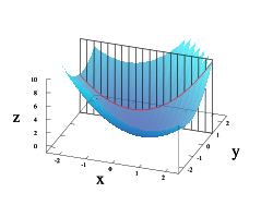
Suppose that f is a function of more than one variable. For instance,

$${\displaystyle z=f(x,y)=x^{2}+xy+y^{2}.}$$

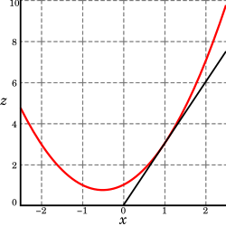
A graph of z = x² + xy + y². For the partial derivative at (1, 1) that leaves y constant, the corresponding tangent line is parallel to the xz-plane.

A slice of the graph above showing the function in the xz-plane at y = 1. The two axes are shown here with different scales. The slope of the tangent line is 3.

The graph of this function defines a surface in Euclidean space. To every point on this surface, there are an infinite number of tangent lines. Partial differentiation is the act of choosing one of these lines and finding its slope. Usually, the lines of most interest are those that are parallel to the xz-plane, and those that are parallel to the yz-plane (which result from holding either y or x constant, respectively).

To find the slope of the line tangent to the function at P(1, 1) and parallel to the xz-plane, we treat y as a constant. The graph and this plane are shown on the right. Below, we see how the function looks on the plane y = 1. By finding the derivative of the equation while assuming that y is a constant, we find that the slope of f at the point (x, y) is:

$${\displaystyle {\frac {\partial z}{\partial x}}=2x+y.}$$

So at (1, 1), by substitution, the slope is 3. Therefore,

$${\displaystyle {\frac {\partial z}{\partial x}}=3}$$

at the point (1, 1). That is, the partial derivative of z with respect to x at (1, 1) is 3, as shown in the graph.

The function f can be reinterpreted as a family of functions of one variable indexed by the other variables:

$${\displaystyle f(x,y)=f_{y}(x)=x^{2}+xy+y^{2}.}$$

In other words, every value of y defines a function, denoted f_y, which is a function of one variable x. ^[6] That is,

$${\displaystyle f_{y}(x)=x^{2}+xy+y^{2}.}$$

In this section the subscript notation f_y denotes a function contingent on a fixed value of y, and not a partial derivative.

Once a value of y is chosen, say a, then f(x,y) determines a function f_a which traces a curve x² + ax + a² on the xz-plane:

$${\displaystyle f_{a}(x)=x^{2}+ax+a^{2}.}$$

In this expression, a is a constant, not a variable, so f_a is a function of only one real variable, that being x. Consequently, the definition of the derivative for a function of one variable applies:

$${\displaystyle f_{a}'(x)=2x+a.}$$

The above procedure can be performed for any choice of a. Assembling the derivatives together into a function gives a function which describes the variation of f in the x direction:

$${\displaystyle {\frac {\partial f}{\partial x}}(x,y)=2x+y.}$$

This is the partial derivative of f with respect to x. Here '∂' is a rounded 'd' called the partial derivative symbol ; to distinguish it from the letter 'd', '∂' is sometimes pronounced "partial".

Higher order partial derivatives

Second and higher order partial derivatives are defined analogously to the higher order derivatives of univariate functions. For the function ${\displaystyle f(x,y,...)}$ the "own" second partial derivative with respect to x is simply the partial derivative of the partial derivative (both with respect to x): ^{[7] : 316–318}

$${\displaystyle {\frac {\partial ^{2}f}{\partial x^{2}}}\equiv \partial {\frac {\partial f/\partial x}{\partial x}}\equiv {\frac {\partial f_{x}}{\partial x}}\equiv f_{xx}.}$$

The cross partial derivative with respect to x and y is obtained by taking the partial derivative of f with respect to x, and then taking the partial derivative of the result with respect to y, to obtain

$${\displaystyle {\frac {\partial ^{2}f}{\partial y\,\partial x}}\equiv \partial {\frac {\partial f/\partial x}{\partial y}}\equiv {\frac {\partial f_{x}}{\partial y}}\equiv f_{xy}.}$$

Schwarz's theorem states that if the second derivatives are continuous, the expression for the cross partial derivative is unaffected by which variable the partial derivative is taken with respect to first and which is taken second. That is,

$${\displaystyle {\frac {\partial ^{2}f}{\partial x\,\partial y}}={\frac {\partial ^{2}f}{\partial y\,\partial x}}}$$

or equivalently ${\displaystyle f_{yx}=f_{xy}.}$

Own and cross partial derivatives appear in the Hessian matrix which is used in the second order conditions in optimization problems. The higher order partial derivatives can be obtained by successive differentiation

Antiderivative analogue

There is a concept for partial derivatives that is analogous to antiderivatives for regular derivatives. Given a partial derivative, it allows for the partial recovery of the original function.

Consider the example of

$${\displaystyle {\frac {\partial z}{\partial x}}=2x+y.}$$

The so-called partial integral can be taken with respect to x (treating y as constant, in a similar manner to partial differentiation):

$${\displaystyle z=\int {\frac {\partial z}{\partial x}}\,dx=x^{2}+xy+g(y).}$$

Here, the constant of integration is no longer a constant, but instead a function of all the variables of the original function except x. The reason for this is that all the other variables are treated as constant when taking the partial derivative, so any function which does not involve x will disappear when taking the partial derivative, and we have to account for this when we take the antiderivative. The most general way to represent this is to have the constant represent an unknown function of all the other variables.

Thus the set of functions ${\displaystyle x^{2}+xy+g(y)}$, where g is any one-argument function, represents the entire set of functions in variables x, y that could have produced the x-partial derivative ${\displaystyle 2x+y}$.

If all the partial derivatives of a function are known (for example, with the gradient), then the antiderivatives can be matched via the above process to reconstruct the original function up to a constant. Unlike in the single-variable case, however, not every set of functions can be the set of all (first) partial derivatives of a single function. In other words, not every vector field is conservative.

Applications

Geometry

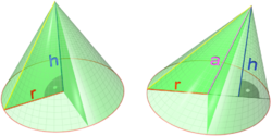
The volume of a cone depends on height and radius

The volume V of a cone depends on the cone's height h and its radius r according to the formula

$${\displaystyle V(r,h)={\frac {\pi r^{2}h}{3}}.}$$

The partial derivative of V with respect to r is

$${\displaystyle {\frac {\partial V}{\partial r}}={\frac {2\pi rh}{3}},}$$

which represents the rate with which a cone's volume changes if its radius is varied and its height is kept constant. The partial derivative with respect to h equals ${\textstyle {\frac {1}{3}}\pi r^{2}}$, which represents the rate with which the volume changes if its height is varied and its radius is kept constant.

By contrast, the total derivative of V with respect to r and h are respectively

$${\displaystyle {\begin{aligned}{\frac {dV}{dr}}&=\overbrace {\frac {2\pi rh}{3}} ^{\frac {\partial V}{\partial r}}+\overbrace {\frac {\pi r^{2}}{3}} ^{\frac {\partial V}{\partial h}}{\frac {dh}{dr}}\,,\\{\frac {dV}{dh}}&=\overbrace {\frac {\pi r^{2}}{3}} ^{\frac {\partial V}{\partial h}}+\overbrace {\frac {2\pi rh}{3}} ^{\frac {\partial V}{\partial r}}{\frac {dr}{dh}}\,.\end{aligned}}}$$

The difference between the total and partial derivative is the elimination of indirect dependencies between variables in partial derivatives.

If (for some arbitrary reason) the cone's proportions have to stay the same, and the height and radius are in a fixed ratio k,

$${\displaystyle k={\frac {h}{r}}={\frac {dh}{dr}}.}$$

This gives the total derivative with respect to r,

$${\displaystyle {\frac {dV}{dr}}={\frac {2\pi rh}{3}}+{\frac {\pi r^{2}}{3}}k\,,}$$

which simplifies to

$${\displaystyle {\frac {dV}{dr}}=k\pi r^{2},}$$

Similarly, the total derivative with respect to h is

$${\displaystyle {\frac {dV}{dh}}=\pi r^{2}.}$$

The total derivative with respect to bothr and h of the volume intended as scalar function of these two variables is given by the gradient vector

$${\displaystyle \nabla V=\left({\frac {\partial V}{\partial r}},{\frac {\partial V}{\partial h}}\right)=\left({\frac {2}{3}}\pi rh,{\frac {1}{3}}\pi r^{2}\right).}$$

Optimization

Partial derivatives appear in any calculus-based optimization problem with more than one choice variable. For example, in economics a firm may wish to maximize profit π(x, y) with respect to the choice of the quantities x and y of two different types of output. The first order conditions for this optimization are π_x = 0 = π_y. Since both partial derivatives π_x and π_y will generally themselves be functions of both arguments x and y, these two first order conditions form a system of two equations in two unknowns.

Thermodynamics, quantum mechanics and mathematical physics

Partial derivatives appear in thermodynamic equations like Gibbs-Duhem equation, in quantum mechanics as in Schrödinger wave equation, as well as in other equations from mathematical physics. The variables being held constant in partial derivatives here can be ratios of simple variables like mole fractions x_i in the following example involving the Gibbs energies in a ternary mixture system:

$${\displaystyle {\bar {G_{2}}}=G+(1-x_{2})\left({\frac {\partial G}{\partial x_{2}}}\right)_{\frac {x_{1}}{x_{3}}}}$$

Express mole fractions of a component as functions of other components' mole fraction and binary mole ratios:

${\textstyle {\begin{aligned}x_{1}&={\frac {1-x_{2}}{1+{\frac {x_{3}}{x_{1}}}}}\\x_{3}&={\frac {1-x_{2}}{1+{\frac {x_{1}}{x_{3}}}}}\end{aligned}}}$

Differential quotients can be formed at constant ratios like those above:

$${\displaystyle {\begin{aligned}\left({\frac {\partial x_{1}}{\partial x_{2}}}\right)_{\frac {x_{1}}{x_{3}}}&=-{\frac {x_{1}}{1-x_{2}}}\\\left({\frac {\partial x_{3}}{\partial x_{2}}}\right)_{\frac {x_{1}}{x_{3}}}&=-{\frac {x_{3}}{1-x_{2}}}\end{aligned}}}$$

Ratios X, Y, Z of mole fractions can be written for ternary and multicomponent systems:

$${\displaystyle {\begin{aligned}X&={\frac {x_{3}}{x_{1}+x_{3}}}\\Y&={\frac {x_{3}}{x_{2}+x_{3}}}\\Z&={\frac {x_{2}}{x_{1}+x_{2}}}\end{aligned}}}$$

which can be used for solving partial differential equations like:

$${\displaystyle \left({\frac {\partial \mu _{2}}{\partial n_{1}}}\right)_{n_{2},n_{3}}=\left({\frac {\partial \mu _{1}}{\partial n_{2}}}\right)_{n_{1},n_{3}}}$$

This equality can be rearranged to have differential quotient of mole fractions on one side.

Image resizing

Partial derivatives are key to target-aware image resizing algorithms. Widely known as seam carving, these algorithms require each pixel in an image to be assigned a numerical 'energy' to describe their dissimilarity against orthogonal adjacent pixels. The algorithm then progressively removes rows or columns with the lowest energy. The formula established to determine a pixel's energy (magnitude of gradient at a pixel) depends heavily on the constructs of partial derivatives.

Economics

Partial derivatives play a prominent role in economics, in which most functions describing economic behaviour posit that the behaviour depends on more than one variable. For example, a societal consumption function may describe the amount spent on consumer goods as depending on both income and wealth; the marginal propensity to consume is then the partial derivative of the consumption function with respect to income.

See also

• d'Alembert operator
• Chain rule
• Curl (mathematics)
• Divergence
• Exterior derivative
• Iterated integral
• Jacobian matrix and determinant
• Laplace operator
• Multivariable calculus
• Symmetry of second derivatives
• Triple product rule, also known as the cyclic chain rule.

Notes

1. Cajori, Florian (1952), A History of Mathematical Notations, vol. 2 (3 ed.), The Open Court Publishing Company, 596
2. Miller, Jeff (n.d.). "Earliest Uses of Symbols of Calculus". In O'Connor, John J.; Robertson, Edmund F. (eds.). MacTutor History of Mathematics archive . University of St Andrews . Retrieved 2023-06-15.
3. Spivak, M. (1965). Calculus on Manifolds. New York: W. A. Benjamin. p. 44. ISBN   9780805390216.
4. R. Wrede; M.R. Spiegel (2010). Advanced Calculus (3rd ed.). Schaum's Outline Series. ISBN   978-0-07-162366-7.
5. The applicability extends to functions over spaces without a metric and to differentiable manifolds, such as in general relativity.
6. This can also be expressed as the adjointness between the product space and function space constructions.
7. Chiang, Alpha C. (1984). Fundamental Methods of Mathematical Economics (3rd ed.). McGraw-Hill.

External links

• "Partial derivative", Encyclopedia of Mathematics , EMS Press, 2001 [1994]
• Partial Derivatives at MathWorld