Contour integration

This article is about the line integral in the complex plane. For the general line integral, see Line integral.

In the mathematical field of complex analysis, contour integration is a method of evaluating certain integrals along paths in the complex plane. ^{[1] [2] [3]}

Contour integration is closely related to the calculus of residues, ^[4] a method of complex analysis.

One use for contour integrals is the evaluation of integrals along the real line that are not readily found by using only real variable methods. ^[5]

Contour integration methods include:

• direct integration of a complex-valued function along a curve in the complex plane;
• application of the Cauchy integral formula; and
• application of the residue theorem.

One method can be used, or a combination of these methods, or various limiting processes, for the purpose of finding these integrals or sums.

Curves in the complex plane

In complex analysis a contour is a type of curve in the complex plane. In contour integration, contours provide a precise definition of the curves on which an integral may be suitably defined. A curve in the complex plane is defined as a continuous function from a closed interval of the real line to the complex plane: ${\displaystyle z:[a,b]\to \mathbb {C} }$.

This definition of a curve coincides with the intuitive notion of a curve, but includes a parametrization by a continuous function from a closed interval. This more precise definition allows us to consider what properties a curve must have for it to be useful for integration. In the following subsections we narrow down the set of curves that we can integrate to include only those that can be built up out of a finite number of continuous curves that can be given a direction. Moreover, we will restrict the "pieces" from crossing over themselves, and we require that each piece have a finite (non-vanishing) continuous derivative. These requirements correspond to requiring that we consider only curves that can be traced, such as by a pen, in a sequence of even, steady strokes, which stop only to start a new piece of the curve, all without picking up the pen. ^[6]

Directed smooth curves

Contours are often defined in terms of directed smooth curves. ^[6] These provide a precise definition of a "piece" of a smooth curve, of which a contour is made.

A smooth curve is a curve ${\displaystyle z:[a,b]\to \mathbb {C} }$ with a non-vanishing, continuous derivative such that each point is traversed only once (z is one-to-one), with the possible exception of a curve such that the endpoints match (${\displaystyle z(a)=z(b)}$). In the case where the endpoints match the curve is called closed, and the function is required to be one-to-one everywhere else and the derivative must be continuous at the identified point (${\displaystyle z'(a)=z'(b)}$). A smooth curve that is not closed is often referred to as a smooth arc. ^[6]

The parametrization of a curve provides a natural ordering of points on the curve: ${\displaystyle z(x)}$ comes before ${\displaystyle z(y)}$ if ${\displaystyle x<y}$. This leads to the notion of a directed smooth curve. It is most useful to consider curves independent of the specific parametrization. This can be done by considering equivalence classes of smooth curves with the same direction. A directed smooth curve can then be defined as an ordered set of points in the complex plane that is the image of some smooth curve in their natural order (according to the parametrization). Note that not all orderings of the points are the natural ordering of a smooth curve. In fact, a given smooth curve has only two such orderings. Also, a single closed curve can have any point as its endpoint, while a smooth arc has only two choices for its endpoints.

Contours

Contours are the class of curves on which we define contour integration. A contour is a directed curve which is made up of a finite sequence of directed smooth curves whose endpoints are matched to give a single direction. This requires that the sequence of curves ${\displaystyle \gamma _{1},\dots ,\gamma _{n}}$ be such that the terminal point of ${\displaystyle \gamma _{i}}$ coincides with the initial point of ${\displaystyle \gamma _{i+1}}$ for all ${\displaystyle i}$ such that ${\displaystyle 1\leq i<n}$ . This includes all directed smooth curves. Also, a single point in the complex plane is considered a contour. The symbol ${\displaystyle +}$ is often used to denote the piecing of curves together to form a new curve. Thus we could write a contour ${\displaystyle \Gamma }$ that is made up of ${\displaystyle n}$ curves as

$${\displaystyle \Gamma =\gamma _{1}+\gamma _{2}+\cdots +\gamma _{n}.}$$

Contour integrals

The contour integral of a complex function ${\displaystyle f:\mathbb {C} \to \mathbb {C} }$ is a generalization of the integral for real-valued functions. For continuous functions in the complex plane, the contour integral can be defined in analogy to the line integral by first defining the integral along a directed smooth curve in terms of an integral over a real valued parameter. A more general definition can be given in terms of partitions of the contour in analogy with the partition of an interval and the Riemann integral. In both cases the integral over a contour is defined as the sum of the integrals over the directed smooth curves that make up the contour.

For continuous functions

To define the contour integral in this way one must first consider the integral, over a real variable, of a complex-valued function. Let ${\displaystyle f:\mathbb {R} \to \mathbb {C} }$ be a complex-valued function of a real variable, ${\displaystyle t}$. The real and imaginary parts of ${\displaystyle f}$ are often denoted as ${\displaystyle u(t)}$ and ${\displaystyle v(t)}$, respectively, so that

$${\displaystyle f(t)=u(t)+iv(t).}$$

Then the integral of the complex-valued function ${\displaystyle f}$ over the interval ${\displaystyle [a,b]}$ is given by

$${\displaystyle {\begin{aligned}\int _{a}^{b}f(t)\,dt&=\int _{a}^{b}{\big (}u(t)+iv(t){\big )}\,dt\\&=\int _{a}^{b}u(t)\,dt+i\int _{a}^{b}v(t)\,dt.\end{aligned}}}$$

Now, to define the contour integral, let ${\displaystyle f:\mathbb {C} \to \mathbb {C} }$ be a continuous function on the directed smooth curve ${\displaystyle \gamma }$. Let ${\displaystyle z:[a,b]\to \mathbb {C} }$ be any parametrization of ${\displaystyle \gamma }$ that is consistent with its order (direction). Then the integral along ${\displaystyle \gamma }$ is denoted

$${\displaystyle \int _{\gamma }f(z)\,dz\,}$$

and is given by ^[6]

$${\displaystyle \int _{\gamma }f(z)\,dz:=\int _{a}^{b}f{\big (}z(t){\big )}z'(t)\,dt.}$$

This definition is well defined. That is, the result is independent of the parametrization chosen. ^[6] In the case where the real integral on the right side does not exist the integral along ${\displaystyle \gamma }$ is said not to exist.

As a generalization of the Riemann integral

The generalization of the Riemann integral to functions of a complex variable is done in complete analogy to its definition for functions from the real numbers. The partition of a directed smooth curve ${\displaystyle \gamma }$ is defined as a finite, ordered set of points on ${\displaystyle \gamma }$. The integral over the curve is the limit of finite sums of function values, taken at the points on the partition, in the limit that the maximum distance between any two successive points on the partition (in the two-dimensional complex plane), also known as the mesh, goes to zero.

Direct methods

Direct methods involve the calculation of the integral through methods similar to those in calculating line integrals in multivariate calculus. This means that we use the following method:

• parametrizing the contour

  The contour is parametrized by a differentiable complex-valued function of real variables, or the contour is broken up into pieces and parametrized separately.

• substitution of the parametrization into the integrand

  Substituting the parametrization into the integrand transforms the integral into an integral of one real variable.

• direct evaluation

  The integral is evaluated in a method akin to a real-variable integral.

Example

A fundamental result in complex analysis is that the contour integral of 1/z is 2πi, where the path of the contour is taken to be the unit circle traversed counterclockwise (or any positively oriented Jordan curve about 0). In the case of the unit circle there is a direct method to evaluate the integral

$${\displaystyle \oint _{C}{\frac {1}{z}}\,dz.}$$

In evaluating this integral, use the unit circle |z| = 1 as a contour, parametrized by z(t) = e^it, with t ∈ [0, 2π], then dz/dt = ie^it and

$${\displaystyle \oint _{C}{\frac {1}{z}}\,dz=\int _{0}^{2\pi }{\frac {1}{e^{it}}}ie^{it}\,dt=i\int _{0}^{2\pi }1\,dt=i\,t{\Big |}_{0}^{2\pi }=\left(2\pi -0\right)i=2\pi i}$$

which is the value of the integral. This result only applies to the case in which z is raised to power of -1. If the power is not equal to -1, then the result will always be zero.

Applications of integral theorems

Applications of integral theorems are also often used to evaluate the contour integral along a contour, which means that the real-valued integral is calculated simultaneously along with calculating the contour integral.

Integral theorems such as the Cauchy integral formula or residue theorem are generally used in the following method:

• a specific contour is chosen:

  The contour is chosen so that the contour follows the part of the complex plane that describes the real-valued integral, and also encloses singularities of the integrand so application of the Cauchy integral formula or residue theorem is possible

• application of Cauchy's integral theorem

  The integral is reduced to only an integration around a small circle about each pole.

• application of the Cauchy integral formula or residue theorem

  Application of these integral formulae gives us a value for the integral around the whole of the contour.

• division of the contour into a contour along the real part and imaginary part

  The whole of the contour can be divided into the contour that follows the part of the complex plane that describes the real-valued integral as chosen before (call it R), and the integral that crosses the complex plane (call it I). The integral over the whole of the contour is the sum of the integral over each of these contours.

• demonstration that the integral that crosses the complex plane plays no part in the sum

  If the integral I can be shown to be zero, or if the real-valued integral that is sought is improper, then if we demonstrate that the integral I as described above tends to 0, the integral along R will tend to the integral around the contour R + I.

• conclusion

  If we can show the above step, then we can directly calculate R, the real-valued integral.

Example 1

Consider the integral

$${\displaystyle \int _{-\infty }^{\infty }{\frac {1}{\left(x^{2}+1\right)^{2}}}\,dx,}$$

To evaluate this integral, we look at the complex-valued function

$${\displaystyle f(z)={\frac {1}{\left(z^{2}+1\right)^{2}}}}$$

which has singularities at i and −i. We choose a contour that will enclose the real-valued integral, here a semicircle with boundary diameter on the real line (going from, say, −a to a) will be convenient. Call this contour C.

There are two ways of proceeding, using the Cauchy integral formula or by the method of residues:

Using the Cauchy integral formula

Note that:

$${\displaystyle \oint _{C}f(z)\,dz=\int _{-a}^{a}f(z)\,dz+\int _{\text{Arc}}f(z)\,dz}$$

thus

$${\displaystyle \int _{-a}^{a}f(z)\,dz=\oint _{C}f(z)\,dz-\int _{\text{Arc}}f(z)\,dz}$$

Furthermore, observe that

$${\displaystyle f(z)={\frac {1}{\left(z^{2}+1\right)^{2}}}={\frac {1}{(z+i)^{2}(z-i)^{2}}}.}$$

Since the only singularity in the contour is the one at i, then we can write

$${\displaystyle f(z)={\frac {\frac {1}{(z+i)^{2}}}{(z-i)^{2}}},}$$

which puts the function in the form for direct application of the formula. Then, by using Cauchy's integral formula,

$${\displaystyle \oint _{C}f(z)\,dz=\oint _{C}{\frac {\frac {1}{(z+i)^{2}}}{(z-i)^{2}}}\,dz=2\pi i\,\left.{\frac {d}{dz}}{\frac {1}{(z+i)^{2}}}\right|_{z=i}=2\pi i\left[{\frac {-2}{(z+i)^{3}}}\right]_{z=i}={\frac {\pi }{2}}}$$

We take the first derivative, in the above steps, because the pole is a second-order pole. That is, (z − i) is taken to the second power, so we employ the first derivative of f(z). If it were (z − i) taken to the third power, we would use the second derivative and divide by 2!, etc. The case of (z − i) to the first power corresponds to a zero order derivative—just f(z) itself.

We need to show that the integral over the arc of the semicircle tends to zero as a → ∞, using the estimation lemma

$${\displaystyle \left|\int _{\text{Arc}}f(z)\,dz\right|\leq ML}$$

where M is an upper bound on |f(z)| along the arc and L the length of the arc. Now,

$${\displaystyle \left|\int _{\text{Arc}}f(z)\,dz\right|\leq {\frac {a\pi }{\left(a^{2}-1\right)^{2}}}\to 0{\text{ as }}a\to \infty .}$$

So

$${\displaystyle \int _{-\infty }^{\infty }{\frac {1}{\left(x^{2}+1\right)^{2}}}\,dx=\int _{-\infty }^{\infty }f(z)\,dz=\lim _{a\to +\infty }\int _{-a}^{a}f(z)\,dz={\frac {\pi }{2}}.\quad \square }$$

Using the method of residues

Consider the Laurent series of f(z) about i, the only singularity we need to consider. We then have

$${\displaystyle f(z)={\frac {-1}{4(z-i)^{2}}}+{\frac {-i}{4(z-i)}}+{\frac {3}{16}}+{\frac {i}{8}}(z-i)+{\frac {-5}{64}}(z-i)^{2}+\cdots }$$

(See the sample Laurent calculation from Laurent series for the derivation of this series.)

It is clear by inspection that the residue is −i/4, so, by the residue theorem, we have

$${\displaystyle \oint _{C}f(z)\,dz=\oint _{C}{\frac {1}{\left(z^{2}+1\right)^{2}}}\,dz=2\pi i\,\operatorname {Res} _{z=i}f(z)=2\pi i\left(-{\frac {i}{4}}\right)={\frac {\pi }{2}}\quad \square }$$

Thus we get the same result as before.

Contour note

As an aside, a question can arise whether we do not take the semicircle to include the other singularity, enclosing −i. To have the integral along the real axis moving in the correct direction, the contour must travel clockwise, i.e., in a negative direction, reversing the sign of the integral overall.

This does not affect the use of the method of residues by series.

Example 2 – Cauchy distribution

The integral

$${\displaystyle \int _{-\infty }^{\infty }{\frac {e^{itx}}{x^{2}+1}}\,dx}$$

the contour

(which arises in probability theory as a scalar multiple of the characteristic function of the Cauchy distribution) resists the techniques of elementary calculus. We will evaluate it by expressing it as a limit of contour integrals along the contour C that goes along the real line from −a to a and then counterclockwise along a semicircle centered at 0 from a to −a. Take a to be greater than 1, so that the imaginary unit i is enclosed within the curve. The contour integral is

$${\displaystyle \int _{C}{\frac {e^{itz}}{z^{2}+1}}\,dz.}$$

Since e^itz is an entire function (having no singularities at any point in the complex plane), this function has singularities only where the denominator z² + 1 is zero. Since z² + 1 = (z + i)(z − i), that happens only where z = i or z = −i. Only one of those points is in the region bounded by this contour. The residue of f(z) at z = i is

$${\displaystyle \lim _{z\to i}(z-i)f(z)=\lim _{z\to i}(z-i){\frac {e^{itz}}{z^{2}+1}}=\lim _{z\to i}(z-i){\frac {e^{itz}}{(z-i)(z+i)}}=\lim _{z\to i}{\frac {e^{itz}}{z+i}}={\frac {e^{-t}}{2i}}.}$$

According to the residue theorem, then, we have

$${\displaystyle \int _{C}f(z)\,dz=2\pi i\operatorname {Res} _{z=i}f(z)=2\pi i{\frac {e^{-t}}{2i}}=\pi e^{-t}.}$$

The contour C may be split into a "straight" part and a curved arc, so that

$${\displaystyle \int _{\text{straight}}+\int _{\text{arc}}=\pi e^{-t},}$$

and thus

$${\displaystyle \int _{-a}^{a}=\pi e^{-t}-\int _{\text{arc}}.}$$

According to Jordan's lemma, if t > 0 then

$${\displaystyle \int _{\text{arc}}{\frac {e^{itz}}{z^{2}+1}}\,dz\rightarrow 0{\mbox{ as }}a\rightarrow \infty .}$$

Therefore, if t > 0 then

$${\displaystyle \int _{-\infty }^{\infty }{\frac {e^{itx}}{x^{2}+1}}\,dx=\pi e^{-t}.}$$

A similar argument with an arc that winds around −i rather than i shows that if t < 0 then

$${\displaystyle \int _{-\infty }^{\infty }{\frac {e^{itx}}{x^{2}+1}}\,dx=\pi e^{t},}$$

and finally we have this:

$${\displaystyle \int _{-\infty }^{\infty }{\frac {e^{itx}}{x^{2}+1}}\,dx=\pi e^{-|t|}.\quad \square }$$

(If t = 0 then the integral yields immediately to real-valued calculus methods and its value is π.)

Example 3 – trigonometric integrals

Certain substitutions can be made to integrals involving trigonometric functions, so the integral is transformed into a rational function of a complex variable and then the above methods can be used in order to evaluate the integral.

As an example, consider

$${\displaystyle \int _{-\pi }^{\pi }{\frac {1}{1+3(\cos t)^{2}}}\,dt.}$$

We seek to make a substitution of z = e^it. Now, recall

$${\displaystyle \cos t={\frac {1}{2}}\left(e^{it}+e^{-it}\right)={\frac {1}{2}}\left(z+{\frac {1}{z}}\right)}$$

and

$${\displaystyle {\frac {dz}{dt}}=iz,\ dt={\frac {dz}{iz}}.}$$

Taking C to be the unit circle, we substitute to get:

$${\displaystyle {\begin{aligned}\oint _{C}{\frac {1}{1+3\left({\frac {1}{2}}\left(z+{\frac {1}{z}}\right)\right)^{2}}}\,{\frac {dz}{iz}}&=\oint _{C}{\frac {1}{1+{\frac {3}{4}}\left(z+{\frac {1}{z}}\right)^{2}}}{\frac {1}{iz}}\,dz\\&=\oint _{C}{\frac {-i}{z+{\frac {3}{4}}z\left(z+{\frac {1}{z}}\right)^{2}}}\,dz\\&=-i\oint _{C}{\frac {dz}{z+{\frac {3}{4}}z\left(z^{2}+2+{\frac {1}{z^{2}}}\right)}}\\&=-i\oint _{C}{\frac {dz}{z+{\frac {3}{4}}\left(z^{3}+2z+{\frac {1}{z}}\right)}}\\&=-i\oint _{C}{\frac {dz}{{\frac {3}{4}}z^{3}+{\frac {5}{2}}z+{\frac {3}{4z}}}}\\&=-i\oint _{C}{\frac {4}{3z^{3}+10z+{\frac {3}{z}}}}\,dz\\&=-4i\oint _{C}{\frac {dz}{3z^{3}+10z+{\frac {3}{z}}}}\\&=-4i\oint _{C}{\frac {z}{3z^{4}+10z^{2}+3}}\,dz\\&=-4i\oint _{C}{\frac {z}{3\left(z+{\sqrt {3}}i\right)\left(z-{\sqrt {3}}i\right)\left(z+{\frac {i}{\sqrt {3}}}\right)\left(z-{\frac {i}{\sqrt {3}}}\right)}}\,dz\\&=-{\frac {4i}{3}}\oint _{C}{\frac {z}{\left(z+{\sqrt {3}}i\right)\left(z-{\sqrt {3}}i\right)\left(z+{\frac {i}{\sqrt {3}}}\right)\left(z-{\frac {i}{\sqrt {3}}}\right)}}\,dz.\end{aligned}}}$$

The singularities to be considered are at ${\displaystyle {\tfrac {\pm i}{\sqrt {3}}}.}$ Let C₁ be a small circle about ${\displaystyle {\tfrac {i}{\sqrt {3}}},}$ and C₂ be a small circle about ${\displaystyle {\tfrac {-i}{\sqrt {3}}}.}$ Then we arrive at the following:

$${\displaystyle {\begin{aligned}&-{\frac {4i}{3}}\left[\oint _{C_{1}}{\frac {\frac {z}{\left(z+{\sqrt {3}}i\right)\left(z-{\sqrt {3}}i\right)\left(z+{\frac {i}{\sqrt {3}}}\right)}}{z-{\frac {i}{\sqrt {3}}}}}\,dz+\oint _{C_{2}}{\frac {\frac {z}{\left(z+{\sqrt {3}}i\right)\left(z-{\sqrt {3}}i\right)\left(z-{\frac {i}{\sqrt {3}}}\right)}}{z+{\frac {i}{\sqrt {3}}}}}\,dz\right]\\={}&-{\frac {4i}{3}}\left[2\pi i\left[{\frac {z}{\left(z+{\sqrt {3}}i\right)\left(z-{\sqrt {3}}i\right)\left(z+{\frac {i}{\sqrt {3}}}\right)}}\right]_{z={\frac {i}{\sqrt {3}}}}+2\pi i\left[{\frac {z}{\left(z+{\sqrt {3}}i\right)\left(z-{\sqrt {3}}i\right)\left(z-{\frac {i}{\sqrt {3}}}\right)}}\right]_{z=-{\frac {i}{\sqrt {3}}}}\right]\\={}&{\frac {8\pi }{3}}\left[{\frac {\frac {i}{\sqrt {3}}}{\left({\frac {i}{\sqrt {3}}}+{\sqrt {3}}i\right)\left({\frac {i}{\sqrt {3}}}-{\sqrt {3}}i\right)\left({\frac {i}{\sqrt {3}}}+{\frac {i}{\sqrt {3}}}\right)}}+{\frac {-{\frac {i}{\sqrt {3}}}}{\left(-{\frac {i}{\sqrt {3}}}+{\sqrt {3}}i\right)\left(-{\frac {i}{\sqrt {3}}}-{\sqrt {3}}i\right)\left(-{\frac {i}{\sqrt {3}}}-{\frac {i}{\sqrt {3}}}\right)}}\right]\\={}&{\frac {8\pi }{3}}\left[{\frac {\frac {i}{\sqrt {3}}}{\left({\frac {4}{\sqrt {3}}}i\right)\left(-{\frac {2}{i{\sqrt {3}}}}\right)\left({\frac {2}{{\sqrt {3}}i}}\right)}}+{\frac {-{\frac {i}{\sqrt {3}}}}{\left({\frac {2}{\sqrt {3}}}i\right)\left(-{\frac {4}{\sqrt {3}}}i\right)\left(-{\frac {2}{\sqrt {3}}}i\right)}}\right]\\={}&{\frac {8\pi }{3}}\left[{\frac {\frac {i}{\sqrt {3}}}{i\left({\frac {4}{\sqrt {3}}}\right)\left({\frac {2}{\sqrt {3}}}\right)\left({\frac {2}{\sqrt {3}}}\right)}}+{\frac {-{\frac {i}{\sqrt {3}}}}{-i\left({\frac {2}{\sqrt {3}}}\right)\left({\frac {4}{\sqrt {3}}}\right)\left({\frac {2}{\sqrt {3}}}\right)}}\right]\\={}&{\frac {8\pi }{3}}\left[{\frac {\frac {1}{\sqrt {3}}}{\left({\frac {4}{\sqrt {3}}}\right)\left({\frac {2}{\sqrt {3}}}\right)\left({\frac {2}{\sqrt {3}}}\right)}}+{\frac {\frac {1}{\sqrt {3}}}{\left({\frac {2}{\sqrt {3}}}\right)\left({\frac {4}{\sqrt {3}}}\right)\left({\frac {2}{\sqrt {3}}}\right)}}\right]\\={}&{\frac {8\pi }{3}}\left[{\frac {\frac {1}{\sqrt {3}}}{\frac {16}{3{\sqrt {3}}}}}+{\frac {\frac {1}{\sqrt {3}}}{\frac {16}{3{\sqrt {3}}}}}\right]\\={}&{\frac {8\pi }{3}}\left[{\frac {3}{16}}+{\frac {3}{16}}\right]\\={}&\pi .\end{aligned}}}$$

Example 3a – trigonometric integrals, the general procedure

The above method may be applied to all integrals of the type

$${\displaystyle \int _{0}^{2\pi }{\frac {P{\big (}\sin(t),\sin(2t),\ldots ,\cos(t),\cos(2t),\ldots {\big )}}{Q{\big (}\sin(t),\sin(2t),\ldots ,\cos(t),\cos(2t),\ldots {\big )}}}\,dt}$$

where P and Q are polynomials, i.e. a rational function in trigonometric terms is being integrated. Note that the bounds of integration may as well be π and −π, as in the previous example, or any other pair of endpoints 2π apart.

The trick is to use the substitution z = e^it where dz = ie^it dt and hence

$${\displaystyle {\frac {1}{iz}}\,dz=dt.}$$

This substitution maps the interval [0, 2π] to the unit circle. Furthermore,

$${\displaystyle \sin(kt)={\frac {e^{ikt}-e^{-ikt}}{2i}}={\frac {z^{k}-z^{-k}}{2i}}}$$

and

$${\displaystyle \cos(kt)={\frac {e^{ikt}+e^{-ikt}}{2}}={\frac {z^{k}+z^{-k}}{2}}}$$

so that a rational function f(z) in z results from the substitution, and the integral becomes

$${\displaystyle \oint _{|z|=1}f(z){\frac {1}{iz}}\,dz}$$

which is in turn computed by summing the residues of f(z)1/iz inside the unit circle.

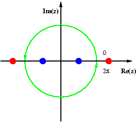
The image at right illustrates this for

$${\displaystyle I=\int _{0}^{\frac {\pi }{2}}{\frac {1}{1+(\sin t)^{2}}}\,dt,}$$

which we now compute. The first step is to recognize that

$${\displaystyle I={\frac {1}{4}}\int _{0}^{2\pi }{\frac {1}{1+(\sin t)^{2}}}\,dt.}$$

The substitution yields

$${\displaystyle {\frac {1}{4}}\oint _{|z|=1}{\frac {4iz}{z^{4}-6z^{2}+1}}\,dz=\oint _{|z|=1}{\frac {iz}{z^{4}-6z^{2}+1}}\,dz.}$$

The poles of this function are at 1 ± √2 and −1 ± √2. Of these, 1 + √2 and −1 − √2 are outside the unit circle (shown in red, not to scale), whereas 1 − √2 and −1 + √2 are inside the unit circle (shown in blue). The corresponding residues are both equal to −i√2/16, so that the value of the integral is

$${\displaystyle I=2\pi i\;2\left(-{\frac {\sqrt {2}}{16}}i\right)=\pi {\frac {\sqrt {2}}{4}}.}$$

Example 4 – branch cuts

Consider the real integral

$${\displaystyle \int _{0}^{\infty }{\frac {\sqrt {x}}{x^{2}+6x+8}}\,dx.}$$

We can begin by formulating the complex integral

$${\displaystyle \int _{C}{\frac {\sqrt {z}}{z^{2}+6z+8}}\,dz=I.}$$

We can use the Cauchy integral formula or residue theorem again to obtain the relevant residues. However, the important thing to note is that z^1/2 = e^{(Log z)/2}, so z^1/2 has a branch cut. This affects our choice of the contour C. Normally the logarithm branch cut is defined as the negative real axis, however, this makes the calculation of the integral slightly more complicated, so we define it to be the positive real axis.

Then, we use the so-called keyhole contour, which consists of a small circle about the origin of radius ε say, extending to a line segment parallel and close to the positive real axis but not touching it, to an almost full circle, returning to a line segment parallel, close, and below the positive real axis in the negative sense, returning to the small circle in the middle.

Note that z = −2 and z = −4 are inside the big circle. These are the two remaining poles, derivable by factoring the denominator of the integrand. The branch point at z = 0 was avoided by detouring around the origin.

Let γ be the small circle of radius ε, Γ the larger, with radius R, then

$${\displaystyle \int _{C}=\int _{\varepsilon }^{R}+\int _{\Gamma }+\int _{R}^{\varepsilon }+\int _{\gamma }.}$$

It can be shown that the integrals over Γ and γ both tend to zero as ε → 0 and R → ∞, by an estimation argument above, that leaves two terms. Now since z^1/2 = e^{(Log z)/2}, on the contour outside the branch cut, we have gained 2π in argument along γ. (By Euler's identity, e^iπ represents the unit vector, which therefore has π as its log. This π is what is meant by the argument of z. The coefficient of 1/2 forces us to use 2π.) So

$${\displaystyle {\begin{aligned}\int _{R}^{\varepsilon }{\frac {\sqrt {z}}{z^{2}+6z+8}}\,dz&=\int _{R}^{\varepsilon }{\frac {e^{{\frac {1}{2}}\operatorname {Log} z}}{z^{2}+6z+8}}\,dz\\[6pt]&=\int _{R}^{\varepsilon }{\frac {e^{{\frac {1}{2}}(\log |z|+i\arg {z})}}{z^{2}+6z+8}}\,dz\\[6pt]&=\int _{R}^{\varepsilon }{\frac {e^{{\frac {1}{2}}\log |z|}e^{{\frac {1}{2}}(2\pi i)}}{z^{2}+6z+8}}\,dz\\[6pt]&=\int _{R}^{\varepsilon }{\frac {e^{{\frac {1}{2}}\log |z|}e^{\pi i}}{z^{2}+6z+8}}\,dz\\[6pt]&=\int _{R}^{\varepsilon }{\frac {-{\sqrt {z}}}{z^{2}+6z+8}}\,dz\\[6pt]&=\int _{\varepsilon }^{R}{\frac {\sqrt {z}}{z^{2}+6z+8}}\,dz.\end{aligned}}}$$

Therefore:

$${\displaystyle \int _{C}{\frac {\sqrt {z}}{z^{2}+6z+8}}\,dz=2\int _{0}^{\infty }{\frac {\sqrt {x}}{x^{2}+6x+8}}\,dx.}$$

By using the residue theorem or the Cauchy integral formula (first employing the partial fractions method to derive a sum of two simple contour integrals) one obtains

$${\displaystyle \pi i\left({\frac {i}{\sqrt {2}}}-i\right)=\int _{0}^{\infty }{\frac {\sqrt {x}}{x^{2}+6x+8}}\,dx=\pi \left(1-{\frac {1}{\sqrt {2}}}\right).\quad \square }$$

Example 5 – the square of the logarithm

This section treats a type of integral of which

$${\displaystyle \int _{0}^{\infty }{\frac {\log x}{\left(1+x^{2}\right)^{2}}}\,dx}$$

is an example.

To calculate this integral, one uses the function

$${\displaystyle f(z)=\left({\frac {\log z}{1+z^{2}}}\right)^{2}}$$

and the branch of the logarithm corresponding to −π < arg z ≤ π.

We will calculate the integral of f(z) along the keyhole contour shown at right. As it turns out this integral is a multiple of the initial integral that we wish to calculate and by the Cauchy residue theorem we have

$${\displaystyle {\begin{aligned}\left(\int _{R}+\int _{M}+\int _{N}+\int _{r}\right)f(z)\,dz&=2\pi i{\big (}\operatorname {Res} _{z=i}f(z)+\operatorname {Res} _{z=-i}f(z){\big )}\\&=2\pi i\left(-{\frac {\pi }{4}}+{\frac {1}{16}}i\pi ^{2}-{\frac {\pi }{4}}-{\frac {1}{16}}i\pi ^{2}\right)\\&=-i\pi ^{2}.\end{aligned}}}$$

Let R be the radius of the large circle, and r the radius of the small one. We will denote the upper line by M, and the lower line by N. As before we take the limit when R → ∞ and r → 0. The contributions from the two circles vanish. For example, one has the following upper bound with the ML lemma:

$${\displaystyle \left|\int _{R}f(z)\,dz\right|\leq 2\pi R{\frac {(\log R)^{2}+\pi ^{2}}{\left(R^{2}-1\right)^{2}}}\to 0.}$$

In order to compute the contributions of M and N we set z = −x + iε on M and z = −x − iε on N, with 0 < x < ∞:

$${\displaystyle {\begin{aligned}-i\pi ^{2}&=\left(\int _{R}+\int _{M}+\int _{N}+\int _{r}\right)f(z)\,dz\\[6pt]&=\left(\int _{M}+\int _{N}\right)f(z)\,dz&&\int _{R},\int _{r}{\mbox{ vanish}}\\[6pt]&=-\int _{\infty }^{0}\left({\frac {\log(-x+i\varepsilon )}{1+(-x+i\varepsilon )^{2}}}\right)^{2}\,dx-\int _{0}^{\infty }\left({\frac {\log(-x-i\varepsilon )}{1+(-x-i\varepsilon )^{2}}}\right)^{2}\,dx\\[6pt]&=\int _{0}^{\infty }\left({\frac {\log(-x+i\varepsilon )}{1+(-x+i\varepsilon )^{2}}}\right)^{2}\,dx-\int _{0}^{\infty }\left({\frac {\log(-x-i\varepsilon )}{1+(-x-i\varepsilon )^{2}}}\right)^{2}\,dx\\[6pt]&=\int _{0}^{\infty }\left({\frac {\log x+i\pi }{1+x^{2}}}\right)^{2}\,dx-\int _{0}^{\infty }\left({\frac {\log x-i\pi }{1+x^{2}}}\right)^{2}\,dx&&\varepsilon \to 0\\&=\int _{0}^{\infty }{\frac {(\log x+i\pi )^{2}-(\log x-i\pi )^{2}}{\left(1+x^{2}\right)^{2}}}\,dx\\[6pt]&=\int _{0}^{\infty }{\frac {4\pi i\log x}{\left(1+x^{2}\right)^{2}}}\,dx\\[6pt]&=4\pi i\int _{0}^{\infty }{\frac {\log x}{\left(1+x^{2}\right)^{2}}}\,dx\end{aligned}}}$$

which gives

$${\displaystyle \int _{0}^{\infty }{\frac {\log x}{\left(1+x^{2}\right)^{2}}}\,dx=-{\frac {\pi }{4}}.}$$

Example 6 – logarithms and the residue at infinity

We seek to evaluate

$${\displaystyle I=\int _{0}^{3}{\frac {x^{\frac {3}{4}}(3-x)^{\frac {1}{4}}}{5-x}}\,dx.}$$

This requires a close study of

$${\displaystyle f(z)=z^{\frac {3}{4}}(3-z)^{\frac {1}{4}}.}$$

We will construct f(z) so that it has a branch cut on [0, 3], shown in red in the diagram. To do this, we choose two branches of the logarithm, setting

$${\displaystyle z^{\frac {3}{4}}=\exp \left({\frac {3}{4}}\log z\right)\quad {\mbox{where }}-\pi \leq \arg z<\pi }$$

and

$${\displaystyle (3-z)^{\frac {1}{4}}=\exp \left({\frac {1}{4}}\log(3-z)\right)\quad {\mbox{where }}0\leq \arg(3-z)<2\pi .}$$

The cut of z^3⁄4 is therefore (−∞, 0] and the cut of (3 − z)^1/4 is (−∞, 3]. It is easy to see that the cut of the product of the two, i.e. f(z), is [0, 3], because f(z) is actually continuous across (−∞, 0). This is because when z = −r < 0 and we approach the cut from above, f(z) has the value

$${\displaystyle r^{\frac {3}{4}}e^{{\frac {3}{4}}\pi i}(3+r)^{\frac {1}{4}}e^{{\frac {2}{4}}\pi i}=r^{\frac {3}{4}}(3+r)^{\frac {1}{4}}e^{{\frac {5}{4}}\pi i}.}$$

When we approach from below, f(z) has the value

$${\displaystyle r^{\frac {3}{4}}e^{-{\frac {3}{4}}\pi i}(3+r)^{\frac {1}{4}}e^{{\frac {0}{4}}\pi i}=r^{\frac {3}{4}}(3+r)^{\frac {1}{4}}e^{-{\frac {3}{4}}\pi i}.}$$

But

$${\displaystyle e^{-{\frac {3}{4}}\pi i}=e^{{\frac {5}{4}}\pi i},}$$

so that we have continuity across the cut. This is illustrated in the diagram, where the two black oriented circles are labelled with the corresponding value of the argument of the logarithm used in z^3⁄4 and (3 − z)^1/4.

We will use the contour shown in green in the diagram. To do this we must compute the value of f(z) along the line segments just above and just below the cut.

Let z = r (in the limit, i.e. as the two green circles shrink to radius zero), where 0 ≤ r ≤ 3. Along the upper segment, we find that f(z) has the value

$${\displaystyle r^{\frac {3}{4}}e^{{\frac {0}{4}}\pi i}(3-r)^{\frac {1}{4}}e^{{\frac {2}{4}}\pi i}=ir^{\frac {3}{4}}(3-r)^{\frac {1}{4}}}$$

and along the lower segment,

$${\displaystyle r^{\frac {3}{4}}e^{{\frac {0}{4}}\pi i}(3-r)^{\frac {1}{4}}e^{{\frac {0}{4}}\pi i}=r^{\frac {3}{4}}(3-r)^{\frac {1}{4}}.}$$

It follows that the integral of f(z)/5 − z along the upper segment is −iI in the limit, and along the lower segment, I.

If we can show that the integrals along the two green circles vanish in the limit, then we also have the value of I, by the Cauchy residue theorem. Let the radius of the green circles be ρ, where ρ < 0.001 and ρ → 0, and apply the ML inequality. For the circle C_L on the left, we find

$${\displaystyle \left|\int _{C_{\mathrm {L} }}{\frac {f(z)}{5-z}}dz\right|\leq 2\pi \rho {\frac {\rho ^{\frac {3}{4}}3.001^{\frac {1}{4}}}{4.999}}\in {\mathcal {O}}\left(\rho ^{\frac {7}{4}}\right)\to 0.}$$

Similarly, for the circle C_R on the right, we have

$${\displaystyle \left|\int _{C_{\mathrm {R} }}{\frac {f(z)}{5-z}}dz\right|\leq 2\pi \rho {\frac {3.001^{\frac {3}{4}}\rho ^{\frac {1}{4}}}{1.999}}\in {\mathcal {O}}\left(\rho ^{\frac {5}{4}}\right)\to 0.}$$

Now using the Cauchy residue theorem, we have

$${\displaystyle (-i+1)I=-2\pi i\left(\operatorname {Res} _{z=5}{\frac {f(z)}{5-z}}+\operatorname {Res} _{z=\infty }{\frac {f(z)}{5-z}}\right).}$$

where the minus sign is due to the clockwise direction around the residues. Using the branch of the logarithm from before, clearly

$${\displaystyle \operatorname {Res} _{z=5}{\frac {f(z)}{5-z}}=-5^{\frac {3}{4}}e^{{\frac {1}{4}}\log(-2)}.}$$

The pole is shown in blue in the diagram. The value simplifies to

$${\displaystyle -5^{\frac {3}{4}}e^{{\frac {1}{4}}(\log 2+\pi i)}=-e^{{\frac {1}{4}}\pi i}5^{\frac {3}{4}}2^{\frac {1}{4}}.}$$

We use the following formula for the residue at infinity:

$${\displaystyle \operatorname {Res} _{z=\infty }h(z)=\operatorname {Res} _{z=0}\left(-{\frac {1}{z^{2}}}h\left({\frac {1}{z}}\right)\right).}$$

Substituting, we find

$${\displaystyle {\frac {1}{5-{\frac {1}{z}}}}=-z\left(1+5z+5^{2}z^{2}+5^{3}z^{3}+\cdots \right)}$$

and

$${\displaystyle \left({\frac {1}{z^{3}}}\left(3-{\frac {1}{z}}\right)\right)^{\frac {1}{4}}={\frac {1}{z}}(3z-1)^{\frac {1}{4}}={\frac {1}{z}}e^{{\frac {1}{4}}\pi i}(1-3z)^{\frac {1}{4}},}$$

where we have used the fact that −1 = e^πi for the second branch of the logarithm. Next we apply the binomial expansion, obtaining

$${\displaystyle {\frac {1}{z}}e^{{\frac {1}{4}}\pi i}\left(1-{1/4 \choose 1}3z+{1/4 \choose 2}3^{2}z^{2}-{1/4 \choose 3}3^{3}z^{3}+\cdots \right).}$$

The conclusion is that

$${\displaystyle \operatorname {Res} _{z=\infty }{\frac {f(z)}{5-z}}=e^{{\frac {1}{4}}\pi i}\left(5-{\frac {3}{4}}\right)=e^{{\frac {1}{4}}\pi i}{\frac {17}{4}}.}$$

Finally, it follows that the value of I is

$${\displaystyle I=2\pi i{\frac {e^{{\frac {1}{4}}\pi i}}{-1+i}}\left({\frac {17}{4}}-5^{\frac {3}{4}}2^{\frac {1}{4}}\right)=2\pi 2^{-{\frac {1}{2}}}\left({\frac {17}{4}}-5^{\frac {3}{4}}2^{\frac {1}{4}}\right)}$$

which yields

$${\displaystyle I={\frac {\pi }{2{\sqrt {2}}}}\left(17-5^{\frac {3}{4}}2^{\frac {9}{4}}\right)={\frac {\pi }{2{\sqrt {2}}}}\left(17-40^{\frac {3}{4}}\right).}$$

Evaluation with residue theorem

Using the residue theorem, we can evaluate closed contour integrals. The following are examples on evaluating contour integrals with the residue theorem.

Using the residue theorem, let us evaluate this contour integral.

$${\displaystyle \oint _{C}{\frac {e^{z}}{z^{3}}}\,dz}$$

As a refresher, the residue theorem states

$${\displaystyle \oint _{C}f(z)=2\pi i\cdot \sum \operatorname {Res} (f,a_{k}),}$$

where ${\displaystyle \operatorname {Res} }$ is the residue of ${\displaystyle f(z)}$.

${\displaystyle f(z)}$ has only one pole, ${\displaystyle 0}$. From that, we determine that the residue of ${\displaystyle f(z)}$ to be ${\displaystyle {\tfrac {1}{2}}}$

$${\displaystyle {\begin{aligned}\oint _{C}f(z)&=\oint _{C}{\frac {e^{z}}{z^{3}}}\\&=2\pi i\cdot \operatorname {Res} _{z=0}f(z)\\&=2\pi i\operatorname {Res} _{z=0}{\frac {e^{z}}{z^{3}}}\\&=2\pi i\cdot {\frac {1}{2}}\\&=\pi i\end{aligned}}}$$

Thus, using the residue theorem, we can determine:

$${\displaystyle \oint _{C}{\frac {e^{z}}{z^{3}}}dz=\pi i.}$$

Multivariable contour integrals

To solve multivariable contour integrals (i.e. surface integrals, complex volume integrals, and higher order integrals), we must use the divergence theorem. For right now, let ${\displaystyle \nabla }$ be interchangeable with ${\displaystyle \operatorname {Div} }$. These will both serve as the divergence of the vector field denoted as ${\displaystyle \mathbf {F} }$. This theorem states:

$${\displaystyle \underbrace {\int \cdots \int _{U}} _{n}\operatorname {div} (\mathbf {F} )\,dV=\underbrace {\oint \cdots \oint _{\partial U}} _{n-1}\mathbf {F} \cdot \mathbf {n} \,dS}$$

In addition, we also need to evaluate ${\displaystyle \nabla \cdot \mathbf {F} }$ where ${\displaystyle \nabla \cdot \mathbf {F} }$ is an alternate notation of ${\displaystyle \operatorname {div} (\mathbf {F} )}$. The divergence of any dimension can be described as

$${\displaystyle {\begin{aligned}\operatorname {div} (\mathbf {F} )&=\nabla \cdot \mathbf {F} \\&=\left({\frac {\partial }{\partial u}},{\frac {\partial }{\partial x}},{\frac {\partial }{\partial y}},{\frac {\partial }{\partial z}},\dots \right)\cdot (F_{u},F_{x},F_{y},F_{z},\dots )\\&=\left({\frac {\partial F_{u}}{\partial u}}+{\frac {\partial F_{x}}{\partial x}}+{\frac {\partial F_{y}}{\partial y}}+{\frac {\partial F_{z}}{\partial z}}+\cdots \right)\end{aligned}}}$$

Example 1

Let the vector field ${\displaystyle \mathbf {F} =\sin(2x)\mathbf {e} _{x}+\sin(2y)\mathbf {e} _{y}+\sin(2z)\mathbf {e} _{z}}$ and be bounded by the following

$${\displaystyle {0\leq x\leq 1}\quad {0\leq y\leq 3}\quad {-1\leq z\leq 4}}$$

The corresponding double contour integral would be set up as such:

${\displaystyle }$${\displaystyle {\scriptstyle S}}$${\displaystyle \mathbf {F} \cdot \mathbf {n} \,dS}$

We now evaluate ${\displaystyle \nabla \cdot \mathbf {F} }$. Meanwhile, set up the corresponding triple integral:

$${\displaystyle {\begin{aligned}&=\iiint _{V}\left({\frac {\partial F_{x}}{\partial x}}+{\frac {\partial F_{y}}{\partial y}}+{\frac {\partial F_{z}}{\partial z}}\right)dV\\[6pt]&=\iiint _{V}\left({\frac {\partial \sin(2x)}{\partial x}}+{\frac {\partial \sin(2y)}{\partial y}}+{\frac {\partial \sin(2z)}{\partial z}}\right)dV\\[6pt]&=\iiint _{V}2\left(\cos(2x)+\cos(2y)+\cos(2z)\right)dV\\[6pt]&=\int _{0}^{1}\int _{0}^{3}\int _{-1}^{4}2(\cos(2x)+\cos(2y)+\cos(2z))\,dx\,dy\,dz\\[6pt]&=\int _{0}^{1}\int _{0}^{3}(10\cos(2y)+\sin(8)+\sin(2)+10\cos(z))\,dy\,dz\\[6pt]&=\int _{0}^{1}(30\cos(2z)+3\sin(2)+3\sin(8)+5\sin(6))\,dz\\[6pt]&=18\sin(2)+3\sin(8)+5\sin(6)\end{aligned}}}$$

Example 2

Let the vector field ${\displaystyle \mathbf {F} =u^{4}\mathbf {e} _{u}+x^{5}\mathbf {e} _{x}+y^{6}\mathbf {e} _{y}+z^{-3}\mathbf {e} _{z}}$, and remark that there are 4 parameters in this case. Let this vector field be bounded by the following:

$${\displaystyle {0\leq x\leq 1}\quad {-10\leq y\leq 2\pi }\quad {4\leq z\leq 5}\quad {-1\leq u\leq 3}}$$

To evaluate this, we must utilize the divergence theorem as stated before, and we must evaluate ${\displaystyle \nabla \cdot \mathbf {F} }$. Let ${\displaystyle dV=dx\,dy\,dz\,du}$

${\displaystyle {\scriptstyle S}}$${\displaystyle \mathbf {F} \cdot \mathbf {n} \,dS}$

$${\displaystyle {\begin{aligned}&=\iiiint _{V}\left({\frac {\partial F_{u}}{\partial u}}+{\frac {\partial F_{x}}{\partial x}}+{\frac {\partial F_{y}}{\partial y}}+{\frac {\partial F_{z}}{\partial z}}\right)\,dV\\[6pt]&=\iiiint _{V}\left({\frac {\partial u^{4}}{\partial u}}+{\frac {\partial x^{5}}{\partial x}}+{\frac {\partial y^{6}}{\partial y}}+{\frac {\partial z^{-3}}{\partial z}}\right)\,dV\\[6pt]&=\iiiint _{V}{\frac {4u^{3}z^{4}+5x^{4}z^{4}+5y^{4}z^{4}-3}{z^{4}}}\,dV\\[6pt]&=\iiiint _{V}{\frac {4u^{3}z^{4}+5x^{4}z^{4}+5y^{4}z^{4}-3}{z^{4}}}\,dV\\[6pt]&=\int _{0}^{1}\int _{-10}^{2\pi }\int _{4}^{5}\int _{-1}^{3}{\frac {4u^{3}z^{4}+5x^{4}z^{4}+5y^{4}z^{4}-3}{z^{4}}}\,dV\\[6pt]&=\int _{0}^{1}\int _{-10}^{2\pi }\int _{4}^{5}\left({\frac {4(3u^{4}z^{3}+3y^{6}+91z^{3}+3)}{3z^{3}}}\right)\,dy\,dz\,du\\[6pt]&=\int _{0}^{1}\int _{-10}^{2\pi }\left(4u^{4}+{\frac {743440}{21}}+{\frac {4}{z^{3}}}\right)\,dz\,du\\[6pt]&=\int _{0}^{1}\left(-{\frac {1}{2\pi ^{2}}}+{\frac {1486880\pi }{21}}+8\pi u^{4}+40u^{4}+{\frac {371720021}{1050}}\right)\,du\\[6pt]&={\frac {371728421}{1050}}+{\frac {14869136\pi ^{3}-105}{210\pi ^{2}}}\\[6pt]&\approx {576468.77}\end{aligned}}}$$

Thus, we can evaluate a contour integral with ${\displaystyle n=4}$. We can use the same method to evaluate contour integrals for any vector field with ${\displaystyle n>4}$ as well.

Integral representation

An integral representation of a function is an expression of the function involving a contour integral. Various integral representations are known for many special functions. Integral representations can be important for theoretical reasons, e.g. giving analytic continuation or functional equations, or sometimes for numerical evaluations.

Hankel's contour

For example, the original definition of the Riemann zeta function ζ(s) via a Dirichlet series,

$${\displaystyle \zeta (s)=\sum _{n=1}^{\infty }{\frac {1}{n^{s}}},}$$

is valid only for Re(s) > 1. But

$${\displaystyle \zeta (s)=-{\frac {\Gamma (1-s)}{2\pi i}}\int _{H}{\frac {(-t)^{s-1}}{e^{t}-1}}dt,}$$

where the integration is done over the Hankel contour H, is valid for all complex s not equal to 1.

See also

• Residue (complex analysis)
• Cauchy principal value
• Poisson integral
• Pochhammer contour

References

1. Stalker, John (1998). Complex Analysis: Fundamentals of the Classical Theory of Functions. Springer. p. 77. ISBN   0-8176-4038-X.
2. Bak, Joseph; Newman, Donald J. (1997). "Chapters 11 & 12". Complex Analysis. Springer. pp. 130–156. ISBN   0-387-94756-6.
3. Krantz, Steven George (1999). "Chapter 2". Handbook of Complex Variables. Springer. ISBN   0-8176-4011-8.
4. Mitrinović, Dragoslav S.; Kečkić, Jovan D. (1984). "Chapter 2". The Cauchy Method of Residues: Theory and Applications. Springer. ISBN   90-277-1623-4.
5. Mitrinović, Dragoslav S.; Kečkić, Jovan D. (1984). "Chapter 5". The Cauchy Method of Residues: Theory and Applications. Springer. ISBN   90-277-1623-4.
6. Saff, Edward B.; Snider, Arthur David (2003). "Chapter 4". Fundamentals of Complex Analysis with Applications to Engineering, Science, and Mathematics (3rd ed.). Prentice Hall. ISBN   0-1390-7874-6.

Further reading

• Titchmarsh, E. C. (1939), The Theory of Functions (2nd ed.), Oxford University Press, ISBN   0-19-853349-7
• Jean Jacquelin, Marko Riedel, Branche univalente ^{[ permanent dead link ]}, Les-Mathematiques.net, in French.
• Marko Riedel et al., Problème d'intégrale, Les-Mathematiques.net, in French.
• Marko Riedel et al., Integral by residue, math.stackexchange.com.
• W W L Chen, Introduction to Complex Analysis
• Various authors, sin límites ni cotas, es.ciencia.matematicas, in Spanish.

External links

• "Complex integration, method of", Encyclopedia of Mathematics , EMS Press, 2001 [1994]