where and the integrands are functions dependent on the derivative of this integral is expressible as
where the partial derivative indicates that inside the integral, only the variation of with is considered in taking the derivative.[1] It is named after Gottfried Leibniz.
In the special case where the functions and are constants and with values that do not depend on this simplifies to:
If is constant and , which is another common situation (for example, in the proof of Cauchy's repeated integration formula), the Leibniz integral rule becomes:
This important result may, under certain conditions, be used to interchange the integral and partial differential operators, and is particularly useful in the differentiation of integral transforms. An example of such is the moment generating function in probability theory, a variation of the Laplace transform, which can be differentiated to generate the moments of a random variable. Whether Leibniz's integral rule applies is essentially a question about the interchange of limits.
General form: differentiation under the integral sign
Theorem—Let be a function such that both and its partial derivative are continuous in and in some region of the -plane, including Also suppose that the functions and are both continuous and both have continuous derivatives for Then, for
Stronger versions of the theorem only require that the partial derivative exist almost everywhere, and not that it be continuous.[2] This formula is the general form of the Leibniz integral rule and can be derived using the fundamental theorem of calculus. The (first) fundamental theorem of calculus is just the particular case of the above formula where is constant, and does not depend on
If both upper and lower limits are taken as constants, then the formula takes the shape of an operator equation:
where is the partial derivative with respect to and is the integral operator with respect to over a fixed interval. That is, it is related to the symmetry of second derivatives, but involving integrals as well as derivatives. This case is also known as the Leibniz integral rule.
The following three basic theorems on the interchange of limits are essentially equivalent:
the interchange of a derivative and an integral (differentiation under the integral sign; i.e., Leibniz integral rule);
the change of order of partial derivatives;
the change of order of integration (integration under the integral sign; i.e., Fubini's theorem).
Figure 1: A vector field F(r, t) defined throughout space, and a surface Σ bounded by curve ∂Σ moving with velocity v over which the field is integrated.
The Leibniz integral rule can be extended to multidimensional integrals. In two and three dimensions, this rule is better known from the field of fluid dynamics as the Reynolds transport theorem:
where is a scalar function, D(t) and ∂D(t) denote a time-varying connected region of R3 and its boundary, respectively, is the Eulerian velocity of the boundary (see Lagrangian and Eulerian coordinates) and dΣ = ndS is the unit normal component of the surfaceelement.
where Ω(t) is a time-varying domain of integration, ω is a p-form, is the vector field of the velocity, denotes the interior product with , dxω is the exterior derivative of ω with respect to the space variables only and is the time derivative of ω.
However, all of these identities can be derived from a most general statement about Lie derivatives:
Here, the ambient manifold on which the differential form lives includes both space and time.
is the region of integration (a submanifold) at a given instant (it does not depend on , since its parametrization as a submanifold defines its position in time),
is the spacetime vector field obtained from adding the unitary vector field in the direction of time to the purely spatial vector field from the previous formulas (i.e, is the spacetime velocity of ),
Something remarkable about this form, is that it can account for the case when changes its shape and size over time, since such deformations are fully determined by .
Measure theory statement
Let be an open subset of , and be a measure space. Suppose satisfies the following conditions:[5][6][2]
is a Lebesgue-integrable function of for each .
For almost all , the partial derivative exists for all .
There is an integrable function such that for all and almost every .
We first prove the case of constant limits of integration a and b.
We use Fubini's theorem to change the order of integration. For every x and h, such that h > 0 and both x and x +h are within [x0,x1], we have:
Note that the integrals at hand are well defined since is continuous at the closed rectangle and thus also uniformly continuous there; thus its integrals by either dt or dx are continuous in the other variable and also integrable by it (essentially this is because for uniformly continuous functions, one may pass the limit through the integration sign, as elaborated below).
Therefore:
Where we have defined:
(we may replace x0 here by any other point between x0 and x)
F is differentiable with derivative , so we can take the limit where h approaches zero. For the left hand side this limit is:
For the right hand side, we get:
And we thus prove the desired result:
Another proof using the bounded convergence theorem
Note that this proof is weaker in the sense that it only shows that fx(x,t) is Lebesgue integrable, but not that it is Riemann integrable. In the former (stronger) proof, if f(x,t) is Riemann integrable, then so is fx(x,t) (and thus is obviously also Lebesgue integrable).
Let
(1)
By the definition of the derivative,
(2)
Substitute equation (1) into equation (2). The difference of two integrals equals the integral of the difference, and 1/h is a constant, so
We now show that the limit can be passed through the integral sign.
We claim that the passage of the limit under the integral sign is valid by the bounded convergence theorem (a corollary of the dominated convergence theorem). For each δ > 0, consider the difference quotient
For t fixed, the mean value theorem implies there exists z in the interval [x, x + δ] such that
Continuity of fx(x, t) and compactness of the domain together imply that fx(x, t) is bounded. The above application of the mean value theorem therefore gives a uniform (independent of ) bound on . The difference quotients converge pointwise to the partial derivative fx by the assumption that the partial derivative exists.
The above argument shows that for every sequence {δn} → 0, the sequence is uniformly bounded and converges pointwise to fx. The bounded convergence theorem states that if a sequence of functions on a set of finite measure is uniformly bounded and converges pointwise, then passage of the limit under the integral is valid. In particular, the limit and integral may be exchanged for every sequence {δn} → 0. Therefore, the limit as δ → 0 may be passed through the integral sign.
Note: This form can be particularly useful if the expression to be differentiated is of the form:
Because does not depend on the limits of integration, it may be moved out from under the integral sign, and the above form may be used with the Product rule, i.e.,
General form with variable limits
Set
where a and b are functions of α that exhibit increments Δa and Δb, respectively, when α is increased by Δα. Then,
A form of the mean value theorem, , where a < ξ < b, may be applied to the first and last integrals of the formula for Δφ above, resulting in
Divide by Δα and let Δα → 0. Notice ξ1 → a and ξ2 → b. We may pass the limit through the integral sign:
again by the bounded convergence theorem. This yields the general form of the Leibniz integral rule,
Alternative proof of the general form with variable limits, using the chain rule
The general form of Leibniz's Integral Rule with variable limits can be derived as a consequence of the basic form of Leibniz's Integral Rule, the multivariable chain rule, and the First Fundamental Theorem of Calculus. Suppose is defined in a rectangle in the plane, for and . Also, assume and the partial derivative are both continuous functions on this rectangle. Suppose are differentiable real valued functions defined on , with values in (i.e. for every ). Now, set
Since the functions are all differentiable (see the remark at the end of the proof), by the Multivariable Chain Rule, it follows that is differentiable, and its derivative is given by the formula:
Now, note that for every , and for every , we have that , because when taking the partial derivative with respect to of , we are keeping fixed in the expression ; thus the basic form of Leibniz's Integral Rule with constant limits of integration applies. Next, by the First Fundamental Theorem of Calculus, we have that ; because when taking the partial derivative with respect to of , the first variable is fixed, so the fundamental theorem can indeed be applied.
Substituting these results into the equation for above gives:
as desired.
There is a technical point in the proof above which is worth noting: applying the Chain Rule to requires that already be differentiable. This is where we use our assumptions about . As mentioned above, the partial derivatives of are given by the formulas and . Since is continuous, its integral is also a continuous function,[7] and since is also continuous, these two results show that both the partial derivatives of are continuous. Since continuity of partial derivatives implies differentiability of the function,[8] is indeed differentiable.
At time t the surface Σ in Figure 1 contains a set of points arranged about a centroid . The function can be written as
with independent of time. Variables are shifted to a new frame of reference attached to the moving surface, with origin at . For a rigidly translating surface, the limits of integration are then independent of time, so:
where the limits of integration confining the integral to the region Σ no longer are time dependent so differentiation passes through the integration to act on the integrand only:
with the velocity of motion of the surface defined by
This equation expresses the material derivative of the field, that is, the derivative with respect to a coordinate system attached to the moving surface. Having found the derivative, variables can be switched back to the original frame of reference. We notice that (see article on curl)
and that Stokes theorem equates the surface integral of the curl over Σ with a line integral over ∂Σ:
The sign of the line integral is based on the right-hand rule for the choice of direction of line element ds. To establish this sign, for example, suppose the field F points in the positive z-direction, and the surface Σ is a portion of the xy-plane with perimeter ∂Σ. We adopt the normal to Σ to be in the positive z-direction. Positive traversal of ∂Σ is then counterclockwise (right-hand rule with thumb along z-axis). Then the integral on the left-hand side determines a positive flux of F through Σ. Suppose Σ translates in the positive x-direction at velocity v. An element of the boundary of Σ parallel to the y-axis, say ds, sweeps out an area vt × ds in time t. If we integrate around the boundary ∂Σ in a counterclockwise sense, vt × ds points in the negative z-direction on the left side of ∂Σ (where ds points downward), and in the positive z-direction on the right side of ∂Σ (where ds points upward), which makes sense because Σ is moving to the right, adding area on the right and losing it on the left. On that basis, the flux of F is increasing on the right of ∂Σ and decreasing on the left. However, the dot productv × F ⋅ ds = −F × v ⋅ ds = −F ⋅ v × ds. Consequently, the sign of the line integral is taken as negative.
If v is a constant,
which is the quoted result. This proof does not consider the possibility of the surface deforming as it moves.
Suppose a and b are constant, and that f(x) involves a parameter α which is constant in the integration but may vary to form different integrals. Assume that f(x, α) is a continuous function of x and α in the compact set {(x, α): α0 ≤ α ≤ α1 and a ≤ x ≤ b}, and that the partial derivative fα(x, α) exists and is continuous. If one defines:
then may be differentiated with respect to α by differentiating under the integral sign, i.e.,
By the Heine–Cantor theorem it is uniformly continuous in that set. In other words, for any ε > 0 there exists Δα such that for all values of x in [a, b],
On the other hand,
Hence φ(α) is a continuous function.
Similarly if exists and is continuous, then for all ε > 0 there exists Δα such that:
Therefore,
where
Now, ε → 0 as Δα → 0, so
This is the formula we set out to prove.
Now, suppose
where a and b are functions of α which take increments Δa and Δb, respectively, when α is increased by Δα. Then,
A form of the mean value theorem, where a < ξ < b, can be applied to the first and last integrals of the formula for Δφ above, resulting in
Dividing by Δα, letting Δα → 0, noticing ξ1 → a and ξ2 → b and using the above derivation for
yields
This is the general form of the Leibniz integral rule.
Examples
Example 1: Fixed limits
Consider the function
The function under the integral sign is not continuous at the point (x, α) = (0, 0), and the function φ(α) has a discontinuity at α = 0 because φ(α) approaches ±π/2 as α → 0±.
If we differentiate φ(α) with respect to α under the integral sign, we get
which is, of course, true for all values of α except α = 0. This may be integrated (with respect to α) to find
Example 2: Variable limits
An example with variable limits:
Applications
Evaluating definite integrals
The formula
can be of use when evaluating certain definite integrals. When used in this context, the Leibniz integral rule for differentiating under the integral sign is also known as Feynman's trick for integration.
Example 3
Consider
Now,
As varies from to , we have
Hence,
Therefore,
Integrating both sides with respect to , we get:
follows from evaluating :
To determine in the same manner, we should need to substitute in a value of greater than 1 in . This is somewhat inconvenient. Instead, we substitute , where . Then,
Therefore,
The definition of is now complete:
The foregoing discussion, of course, does not apply when , since the conditions for differentiability are not met.
Example 4
First we calculate:
The limits of integration being independent of , we have:
On the other hand:
Equating these two relations then yields
In a similar fashion, pursuing yields
Adding the two results then produces
which computes as desired.
This derivation may be generalized. Note that if we define
it can easily be shown that
Given , this integral reduction formula can be used to compute all of the values of for . Integrals like and may also be handled using the Weierstrass substitution.
Example 5
Here, we consider the integral
Differentiating under the integral with respect to , we have
Therefore:
But by definition so and
Example 6
Here, we consider the integral
We introduce a new variable φ and rewrite the integral as
When φ = 1 this equals the original integral. However, this more general integral may be differentiated with respect to :
Now, fix φ, and consider the vector field on defined by . Further, choose the positive oriented parametrization of the unit circle given by , , so that . Then the final integral above is precisely
the line integral of over . By Green's Theorem, this equals the double integral
where is the closed unit disc. Its integrand is identically 0, so is likewise identically zero. This implies that f(φ) is constant. The constant may be determined by evaluating at :
Therefore, the original integral also equals .
Other problems to solve
There are innumerable other integrals that can be solved using the technique of differentiation under the integral sign. For example, in each of the following cases, the original integral may be replaced by a similar integral having a new parameter :
The first integral, the Dirichlet integral, is absolutely convergent for positive α but only conditionally convergent when . Therefore, differentiation under the integral sign is easy to justify when , but proving that the resulting formula remains valid when requires some careful work.
Infinite series
The measure-theoretic version of differentiation under the integral sign also applies to summation (finite or infinite) by interpreting summation as counting measure. An example of an application is the fact that power series are differentiable in their radius of convergence.[citation needed]
Differentiation under the integral sign is mentioned in the late physicistRichard Feynman's best-selling memoir Surely You're Joking, Mr. Feynman! in the chapter "A Different Box of Tools". He describes learning it, while in high school, from an old text, Advanced Calculus (1926), by Frederick S. Woods (who was a professor of mathematics in the Massachusetts Institute of Technology). The technique was not often taught when Feynman later received his formal education in calculus, but using this technique, Feynman was able to solve otherwise difficult integration problems upon his arrival at graduate school at Princeton University:
One thing I never did learn was contour integration. I had learned to do integrals by various methods shown in a book that my high school physics teacher Mr. Bader had given me. One day he told me to stay after class. "Feynman," he said, "you talk too much and you make too much noise. I know why. You're bored. So I'm going to give you a book. You go up there in the back, in the corner, and study this book, and when you know everything that's in this book, you can talk again." So every physics class, I paid no attention to what was going on with Pascal's Law, or whatever they were doing. I was up in the back with this book: "Advanced Calculus", by Woods. Bader knew I had studied "Calculus for the Practical Man" a little bit, so he gave me the real works—it was for a junior or senior course in college. It had Fourier series, Bessel functions, determinants, elliptic functions—all kinds of wonderful stuff that I didn't know anything about. That book also showed how to differentiate parameters under the integral sign—it's a certain operation. It turns out that's not taught very much in the universities; they don't emphasize it. But I caught on how to use that method, and I used that one damn tool again and again. So because I was self-taught using that book, I had peculiar methods of doing integrals. The result was, when guys at MIT or Princeton had trouble doing a certain integral, it was because they couldn't do it with the standard methods they had learned in school. If it was contour integration, they would have found it; if it was a simple series expansion, they would have found it. Then I come along and try differentiating under the integral sign, and often it worked. So I got a great reputation for doing integrals, only because my box of tools was different from everybody else's, and they had tried all their tools on it before giving the problem to me.
In mathematics, the Laplace transform, named after its discoverer Pierre-Simon Laplace, is an integral transform that converts a function of a real variable to a function of a complex variable .
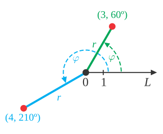
In mathematics, the polar coordinate system is a two-dimensional coordinate system in which each point on a plane is determined by a distance from a reference point and an angle from a reference direction. The reference point is called the pole, and the ray from the pole in the reference direction is the polar axis. The distance from the pole is called the radial coordinate, radial distance or simply radius, and the angle is called the angular coordinate, polar angle, or azimuth. Angles in polar notation are generally expressed in either degrees or radians.
In mathematical analysis, the Dirac delta function, also known as the unit impulse, is a generalized function on the real numbers, whose value is zero everywhere except at zero, and whose integral over the entire real line is equal to one. Since there is no function having this property, to model the delta "function" rigorously involves the use of limits or, as is common in mathematics, measure theory and the theory of distributions.
A Fourier series is an expansion of a periodic function into a sum of trigonometric functions. The Fourier series is an example of a trigonometric series, but not all trigonometric series are Fourier series. By expressing a function as a sum of sines and cosines, many problems involving the function become easier to analyze because trigonometric functions are well understood. For example, Fourier series were first used by Joseph Fourier to find solutions to the heat equation. This application is possible because the derivatives of trigonometric functions fall into simple patterns. Fourier series cannot be used to approximate arbitrary functions, because most functions have infinitely many terms in their Fourier series, and the series do not always converge. Well-behaved functions, for example smooth functions, have Fourier series that converge to the original function. The coefficients of the Fourier series are determined by integrals of the function multiplied by trigonometric functions, described in Common forms of the Fourier series below.
Noether's theorem states that every continuous symmetry of the action of a physical system with conservative forces has a corresponding conservation law. This is the first of two theorems proven by mathematician Emmy Noether in 1915 and published in 1918. The action of a physical system is the integral over time of a Lagrangian function, from which the system's behavior can be determined by the principle of least action. This theorem only applies to continuous and smooth symmetries of physical space.
In mathematics, the Laplace operator or Laplacian is a differential operator given by the divergence of the gradient of a scalar function on Euclidean space. It is usually denoted by the symbols , (where is the nabla operator), or . In a Cartesian coordinate system, the Laplacian is given by the sum of second partial derivatives of the function with respect to each independent variable. In other coordinate systems, such as cylindrical and spherical coordinates, the Laplacian also has a useful form. Informally, the Laplacian Δf (p) of a function f at a point p measures by how much the average value of f over small spheres or balls centered at p deviates from f (p).
In the calculus of variations, a field of mathematical analysis, the functional derivative relates a change in a functional to a change in a function on which the functional depends.
In mathematics, a Green's function is the impulse response of an inhomogeneous linear differential operator defined on a domain with specified initial conditions or boundary conditions.
In geometry, a solid of revolution is a solid figure obtained by rotating a plane figure around some straight line, which may not intersect the generatrix. The surface created by this revolution and which bounds the solid is the surface of revolution.
The path integral formulation is a description in quantum mechanics that generalizes the stationary action principle of classical mechanics. It replaces the classical notion of a single, unique classical trajectory for a system with a sum, or functional integral, over an infinity of quantum-mechanically possible trajectories to compute a quantum amplitude.
In mathematics, the Radon transform is the integral transform which takes a function f defined on the plane to a function Rf defined on the (two-dimensional) space of lines in the plane, whose value at a particular line is equal to the line integral of the function over that line. The transform was introduced in 1917 by Johann Radon, who also provided a formula for the inverse transform. Radon further included formulas for the transform in three dimensions, in which the integral is taken over planes. It was later generalized to higher-dimensional Euclidean spaces and more broadly in the context of integral geometry. The complex analogue of the Radon transform is known as the Penrose transform. The Radon transform is widely applicable to tomography, the creation of an image from the projection data associated with cross-sectional scans of an object.
Arc length is the distance between two points along a section of a curve.
In mathematics (specifically multivariable calculus), a multiple integral is a definite integral of a function of several real variables, for instance, f(x, y) or f(x, y, z). Physical (natural philosophy) interpretation: S any surface, V any volume, etc.. Incl. variable to time, position, etc.
The gradient theorem, also known as the fundamental theorem of calculus for line integrals, says that a line integral through a gradient field can be evaluated by evaluating the original scalar field at the endpoints of the curve. The theorem is a generalization of the second fundamental theorem of calculus to any curve in a plane or space rather than just the real line.
In differential calculus, there is no single uniform notation for differentiation. Instead, various notations for the derivative of a function or variable have been proposed by various mathematicians. The usefulness of each notation varies with the context, and it is sometimes advantageous to use more than one notation in a given context. The most common notations for differentiation are listed below.
In mathematics, vector spherical harmonics (VSH) are an extension of the scalar spherical harmonics for use with vector fields. The components of the VSH are complex-valued functions expressed in the spherical coordinate basis vectors.
Common integrals in quantum field theory are all variations and generalizations of Gaussian integrals to the complex plane and to multiple dimensions. Other integrals can be approximated by versions of the Gaussian integral. Fourier integrals are also considered.
Landen's transformation is a mapping of the parameters of an elliptic integral, useful for the efficient numerical evaluation of elliptic functions. It was originally due to John Landen and independently rediscovered by Carl Friedrich Gauss.
In classical mechanics, the central-force problem is to determine the motion of a particle in a single central potential field. A central force is a force that points from the particle directly towards a fixed point in space, the center, and whose magnitude only depends on the distance of the object to the center. In a few important cases, the problem can be solved analytically, i.e., in terms of well-studied functions such as trigonometric functions.
Lagrangian field theory is a formalism in classical field theory. It is the field-theoretic analogue of Lagrangian mechanics. Lagrangian mechanics is used to analyze the motion of a system of discrete particles each with a finite number of degrees of freedom. Lagrangian field theory applies to continua and fields, which have an infinite number of degrees of freedom.
This page is based on this Wikipedia article Text is available under the CC BY-SA 4.0 license; additional terms may apply. Images, videos and audio are available under their respective licenses.


![Figure 1: A vector field F(r, t) defined throughout space, and a surface S bounded by curve [?]S moving with velocity v over which the field is integrated. Vector field on a surface.svg](http://upload.wikimedia.org/wikipedia/commons/thumb/8/88/Vector_field_on_a_surface.svg/250px-Vector_field_on_a_surface.svg.png)