Lebesgue integration

The integral of a positive function can be interpreted as the area under a curve.

In mathematics, the integral of a non-negative function of a single variable can be regarded, in the simplest case, as the area between the graph of that function and the X axis. The Lebesgue integral, named after French mathematician Henri Lebesgue, extends the integral to a larger class of functions. It also extends the domains on which these functions can be defined.

Long before the 20th century, mathematicians already understood that for non-negative functions with a smooth enough graph—such as continuous functions on closed bounded intervals—the area under the curve could be defined as the integral, and computed using approximation techniques on the region by polygons. However, as the need to consider more irregular functions arose—e.g., as a result of the limiting processes of mathematical analysis and the mathematical theory of probability—it became clear that more careful approximation techniques were needed to define a suitable integral. Also, one might wish to integrate on spaces more general than the real line. The Lebesgue integral provides the necessary abstractions for this.

The Lebesgue integral plays an important role in probability theory, real analysis, and many other fields in mathematics. It is named after Henri Lebesgue (1875–1941), who introduced the integral ( Lebesgue 1904 ). It is also a pivotal part of the axiomatic theory of probability.

The term Lebesgue integration can mean either the general theory of integration of a function with respect to a general measure, as introduced by Lebesgue, or the specific case of integration of a function defined on a sub-domain of the real line with respect to the Lebesgue measure.

Introduction

The integral of a positive real function f between boundaries a and b can be interpreted as the area under the graph of f, between a and b. This notion of area fits some functions, mainly piecewise continuous functions, including elementary functions, for example polynomials. However, the graphs of other functions, for example the Dirichlet function, don't fit well with the notion of area. Graphs like the one of the latter, raise the question: for which class of functions does "area under the curve" make sense? The answer to this question has great theoretical importance.

As part of a general movement toward rigor in mathematics in the nineteenth century, mathematicians attempted to put integral calculus on a firm foundation. The Riemann integral—proposed by Bernhard Riemann (1826–1866)—is a broadly successful attempt to provide such a foundation. Riemann's definition starts with the construction of a sequence of easily calculated areas that converge to the integral of a given function. This definition is successful in the sense that it gives the expected answer for many already-solved problems, and gives useful results for many other problems.

However, Riemann integration does not interact well with taking limits of sequences of functions, making such limiting processes difficult to analyze. This is important, for instance, in the study of Fourier series, Fourier transforms, and other topics. The Lebesgue integral describes better how and when it is possible to take limits under the integral sign (via the monotone convergence theorem and dominated convergence theorem).

While the Riemann integral considers the area under a curve as made out of vertical rectangles, the Lebesgue definition considers horizontal slabs that are not necessarily just rectangles, and so it is more flexible. For this reason, the Lebesgue definition makes it possible to calculate integrals for a broader class of functions. For example, the Dirichlet function, which is 1 where its argument is rational and 0 otherwise, has a Lebesgue integral, but does not have a Riemann integral. Furthermore, the Lebesgue integral of this function is zero, which agrees with the intuition that when picking a real number uniformly at random from the unit interval, the probability of picking a rational number should be zero.

Lebesgue summarized his approach to integration in a letter to Paul Montel:

I have to pay a certain sum, which I have collected in my pocket. I take the bills and coins out of my pocket and give them to the creditor in the order I find them until I have reached the total sum. This is the Riemann integral. But I can proceed differently. After I have taken all the money out of my pocket I order the bills and coins according to identical values and then I pay the several heaps one after the other to the creditor. This is my integral.

— Source: (Siegmund-Schultze 2008)

The insight is that one should be able to rearrange the values of a function freely, while preserving the value of the integral. This process of rearrangement can convert a very pathological function into one that is "nice" from the point of view of integration, and thus let such pathological functions be integrated.

Intuitive interpretation

A measurable function is shown, together with the set {x : f(x) > t} (on the x-axis). The Lebesgue integral is obtained by slicing along the y-axis, using the 1-dimensional Lebesgue measure to measure the "width" of the slices.

Folland (1999) summarizes the difference between the Riemann and Lebesgue approaches thus: "to compute the Riemann integral of f, one partitions the domain [a, b] into subintervals", while in the Lebesgue integral, "one is in effect partitioning the range of f."

For the Riemann integral, the domain is partitioned into intervals, and bars are constructed to meet the height of the graph. The areas of these bars are added together, and this approximates the integral, in effect by summing areas of the form f(x)dx where f(x) is the height of a rectangle and dx is its width.

For the Lebesgue integral, the range is partitioned into intervals, and so the region under the graph is partitioned into horizontal "slabs" (which may not be connected sets). The area of a small horizontal "slab" under the graph of f, of height dy, is equal to the measure of the slab's width times dy:

$${\displaystyle \mu \left(\{x\mid f(x)>y\}\right)\,dy.}$$

The Lebesgue integral may then be defined by adding up the areas of these horizontal slabs. From this perspective, a key difference with the Riemann integral is that the "slabs" are no longer rectangular (cartesian products of two intervals), but instead are cartesian products of a measurable set with an interval.

Simple functions

Riemannian (top) vs Lebesgue (bottom) integration of smoothed COVID-19 daily case data from Serbia (Summer-Fall 2021).

An equivalent way to introduce the Lebesgue integral is to use so-called simple functions, which generalize the step functions of Riemann integration. Consider, for example, determining the cumulative COVID-19 case count from a graph of smoothed cases each day (right).

The Riemann–Darboux approach

Partition the domain (time period) into intervals (eight, in the example at right) and construct bars with heights that meet the graph. The cumulative count is found by summing, over all bars, the product of interval width (time in days) and the bar height (cases per day).

The Lebesgue approach

Choose a finite number of target values (eight, in the example) in the range of the function. By constructing bars with heights equal to these values, but below the function, they imply a partitioning of the domain into the same number of subsets (subsets, indicated by color in the example, need not be connected). This is a "simple function," as described below. The cumulative count is found by summing, over all subsets of the domain, the product of the measure on that subset (total time in days) and the bar height (cases per day).

Measure theory

Further information: Measure (mathematics)

Measure theory was initially created to provide a useful abstraction of the notion of length of subsets of the real line—and, more generally, area and volume of subsets of Euclidean spaces. In particular, it provided a systematic answer to the question of which subsets of R have a length. As later set theory developments showed (see non-measurable set), it is actually impossible to assign a length to all subsets of R in a way that preserves some natural additivity and translation invariance properties. This suggests that picking out a suitable class of measurable subsets is an essential prerequisite.

The Riemann integral uses the notion of length explicitly. Indeed, the element of calculation for the Riemann integral is the rectangle [a, b] × [c, d], whose area is calculated to be (b − a)(d − c). The quantity b − a is the length of the base of the rectangle and d − c is the height of the rectangle. Riemann could only use planar rectangles to approximate the area under the curve, because there was no adequate theory for measuring more general sets.

In the development of the theory in most modern textbooks (after 1950), the approach to measure and integration is axiomatic. This means that a measure is any function μ defined on a certain class X of subsets of a set E, which satisfies a certain list of properties. These properties can be shown to hold in many different cases.

Measurable functions

We start with a measure space (E, X, μ) where E is a set, X is a σ-algebra of subsets of E, and μ is a (non-negative) measure on E defined on the sets of X.

For example, E can be Euclidean n-space Rⁿ or some Lebesgue measurable subset of it, X is the σ-algebra of all Lebesgue measurable subsets of E, and μ is the Lebesgue measure. In the mathematical theory of probability, we confine our study to a probability measure μ, which satisfies μ(E) = 1.

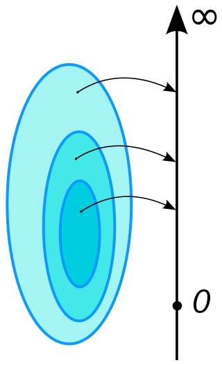
Lebesgue's theory defines integrals for a class of functions called measurable functions. A real-valued function f on E is measurable if the pre-image of every interval of the form (t, ∞) is in X:

$${\displaystyle \{x\,\mid \,f(x)>t\}\in X\quad \forall t\in \mathbb {R} .}$$

We can show that this is equivalent to requiring that the pre-image of any Borel subset of R be in X. The set of measurable functions is closed under algebraic operations, but more importantly it is closed under various kinds of point-wise sequential limits:

$${\displaystyle \sup _{k\in \mathbb {N} }f_{k},\quad \liminf _{k\in \mathbb {N} }f_{k},\quad \limsup _{k\in \mathbb {N} }f_{k}}$$

are measurable if the original sequence (f_k), where k ∈ N, consists of measurable functions.

There are several approaches for defining an integral for measurable real-valued functions f defined on E, and several notations are used to denote such an integral.

$${\displaystyle \int _{E}f\,d\mu =\int _{E}f(x)\,d\mu (x)=\int _{E}f(x)\,\mu (dx).}$$

Following the identification in Distribution theory of measures with distributions of order 0, or with Radon measures, one can also use a dual pair notation and write the integral with respect to μ in the form

$${\displaystyle \langle \mu ,f\rangle .}$$

Definition

The theory of the Lebesgue integral requires a theory of measurable sets and measures on these sets, as well as a theory of measurable functions and integrals on these functions.

Via simple functions

Approximating a function by a simple function.

One approach to constructing the Lebesgue integral is to make use of so-called simple functions: finite, real linear combinations of indicator functions. Simple functions that lie directly underneath a given function f can be constructed by partitioning the range of f into a finite number of layers. The intersection of the graph of f with a layer identifies a set of intervals in the domain of f, which, taken together, is defined to be the preimage of the lower bound of that layer, under the simple function. In this way, the partitioning of the range of f implies a partitioning of its domain. The integral of a simple function is found by summing, over these (not necessarily connected) subsets of the domain, the product of the measure of the subset and its image under the simple function (the lower bound of the corresponding layer); intuitively, this product is the sum of the areas of all bars of the same height. The integral of a non-negative general measurable function is then defined as an appropriate supremum of approximations by simple functions, and the integral of a (not necessarily positive) measurable function is the difference of two integrals of non-negative measurable functions. ^[1]

Indicator functions

To assign a value to the integral of the indicator function 1_S of a measurable set S consistent with the given measure μ, the only reasonable choice is to set:

$${\displaystyle \int 1_{S}\,d\mu =\mu (S).}$$

Notice that the result may be equal to +∞, unless μ is a finite measure.

Simple functions

A finite linear combination of indicator functions

$${\displaystyle \sum _{k}a_{k}1_{S_{k}}}$$

where the coefficients a_k are real numbers and S_k are disjoint measurable sets, is called a measurable simple function. We extend the integral by linearity to non-negative measurable simple functions. When the coefficients a_k are positive, we set

$${\displaystyle \int \left(\sum _{k}a_{k}1_{S_{k}}\right)\,d\mu =\sum _{k}a_{k}\int 1_{S_{k}}\,d\mu =\sum _{k}a_{k}\,\mu (S_{k})}$$

whether this sum is finite or +∞. A simple function can be written in different ways as a linear combination of indicator functions, but the integral will be the same by the additivity of measures.

Some care is needed when defining the integral of a real-valued simple function, to avoid the undefined expression ∞ − ∞: one assumes that the representation

$${\displaystyle f=\sum _{k}a_{k}1_{S_{k}}}$$

is such that μ(S_k) < ∞ whenever a_k ≠ 0. Then the above formula for the integral of f makes sense, and the result does not depend upon the particular representation of f satisfying the assumptions.

If B is a measurable subset of E and s is a measurable simple function one defines

$${\displaystyle \int _{B}s\,\mathrm {d} \mu =\int 1_{B}\,s\,\mathrm {d} \mu =\sum _{k}a_{k}\,\mu (S_{k}\cap B).}$$

Non-negative functions

Let f be a non-negative measurable function on E, which we allow to attain the value +∞, in other words, f takes non-negative values in the extended real number line. We define

$${\displaystyle \int _{E}f\,d\mu =\sup \left\{\,\int _{E}s\,d\mu :0\leq s\leq f,\ s\ {\text{simple}}\,\right\}.}$$

We need to show this integral coincides with the preceding one, defined on the set of simple functions, when E is a segment [a, b]. There is also the question of whether this corresponds in any way to a Riemann notion of integration. It is possible to prove that the answer to both questions is yes.

We have defined the integral of f for any non-negative extended real-valued measurable function on E. For some functions, this integral ${\textstyle \int _{E}f\,d\mu }$ is infinite.

It is often useful to have a particular sequence of simple functions that approximates the Lebesgue integral well (analogously to a Riemann sum). For a non-negative measurable function f, let ${\textstyle s_{n}(x)}$ be the simple function whose value is ${\textstyle k/2^{n}}$ whenever ${\textstyle k/2^{n}\leq f(x)<(k+1)/2^{n}}$, for k a non-negative integer less than, say, ${\textstyle 4^{n}}$. Then it can be proven directly that

$${\displaystyle \int f\,d\mu =\lim _{n\to \infty }\int s_{n}\,d\mu }$$

and that the limit on the right hand side exists as an extended real number. This bridges the connection between the approach to the Lebesgue integral using simple functions, and the motivation for the Lebesgue integral using a partition of the range.

Signed functions

To handle signed functions, we need a few more definitions. If f is a measurable function of the set E to the reals (including ±∞), then we can write

$${\displaystyle f=f^{+}-f^{-},}$$

where

$${\displaystyle {\begin{aligned}f^{+}(x)&={\begin{cases}f(x){\hphantom {-}}&{\text{if }}f(x)>0,\\0&{\text{otherwise}},\end{cases}}\\f^{-}(x)&={\begin{cases}-f(x)&{\text{if }}f(x)<0,\\0&{\text{otherwise}}.\end{cases}}\end{aligned}}}$$

Note that both f⁺ and f⁻ are non-negative measurable functions. Also note that

$${\displaystyle |f|=f^{+}+f^{-}.}$$

We say that the Lebesgue integral of the measurable function fexists, or is defined if at least one of ${\textstyle \int f^{+}\,d\mu }$ and ${\textstyle \int f^{-}\,d\mu }$ is finite:

$${\displaystyle \min \left(\int f^{+}\,d\mu ,\int f^{-}\,d\mu \right)<\infty .}$$

In this case we define

$${\displaystyle \int f\,d\mu =\int f^{+}\,d\mu -\int f^{-}\,d\mu .}$$

If

$${\displaystyle \int |f|\,\mathrm {d} \mu <\infty ,}$$

we say that f is Lebesgue integrable.

It turns out that this definition gives the desirable properties of the integral.

Via improper Riemann integral

See also: Layer cake representation

Assuming that f is measurable and non-negative, the function

$${\displaystyle f^{*}(t)\ {\stackrel {\text{def}}{=}}\ \mu \left(\{x\in E\mid f(x)>t\}\right).}$$

is monotonically non-increasing. The Lebesgue integral may then be defined as the improper Riemann integral of f^∗: ^[2]

$${\displaystyle \int _{E}f\,d\mu \ {\stackrel {\text{def}}{=}}\ \int _{0}^{\infty }f^{*}(t)\,dt.}$$

This integral is improper at the upper limit of ∞, and possibly also at zero. It exists, with the allowance that it may be infinite. ^{[3] [4]}

As above, the integral of a Lebesgue integrable (not necessarily non-negative) function is defined by subtracting the integral of its positive and negative parts.

Complex-valued functions

Complex-valued functions can be similarly integrated, by considering the real part and the imaginary part separately. ^[5]

If h = f + ig for real-valued integrable functions f, g, then the integral of h is defined by

$${\displaystyle \int h\,d\mu =\int f\,d\mu +i\int g\,d\mu .}$$

The function is Lebesgue integrable if and only if its absolute value is Lebesgue integrable (see Absolutely integrable function).

Example

Consider the indicator function of the rational numbers, 1_Q, also known as the Dirichlet function. This function is nowhere continuous.

• ${\displaystyle 1_{\mathbf {Q} }}$is not Riemann-integrable on[ 0, 1]: No matter how the set [ 0, 1] is partitioned into subintervals, each partition contains at least one rational and at least one irrational number, because rationals and irrationals are both dense in the reals. Thus the upper Darboux sums are all one, and the lower Darboux sums are all zero.
• ${\displaystyle 1_{\mathbf {Q} }}$is Lebesgue-integrable on [ 0, 1] using the Lebesgue measure: Indeed, it is the indicator function of the rationals so by definition
  $${\displaystyle \int _{[0,1]}1_{\mathbf {Q} }\,d\mu =\mu (\mathbf {Q} \cap [0,1])=0,}$$
  because Q is countable.

Domain of integration

A technical issue in Lebesgue integration is that the domain of integration is defined as a set (a subset of a measure space), with no notion of orientation. In elementary calculus, one defines integration with respect to an orientation:

$${\displaystyle \int _{b}^{a}f=-\int _{a}^{b}f.}$$

Generalizing this to higher dimensions yields integration of differential forms. By contrast, Lebesgue integration provides an alternative generalization, integrating over subsets with respect to a measure; this can be notated as

$${\displaystyle \int _{A}f\,d\mu =\int _{[a,b]}f\,d\mu }$$

to indicate integration over a subset A. For details on the relation between these generalizations, see Differential form § Relation with measures. The main theory linking these ideas is that of homological integration (sometimes called geometric integration theory), pioneered by Georges de Rham and Hassler Whitney. ^[6]

Limitations of the Riemann integral

With the advent of Fourier series, many analytical problems involving integrals came up whose satisfactory solution required interchanging limit processes and integral signs. However, the conditions under which the integrals

$${\displaystyle \sum _{k}\int f_{k}(x)\,dx,\quad \int \left[\sum _{k}f_{k}(x)\right]dx}$$

are equal proved quite elusive in the Riemann framework. There are some other technical difficulties with the Riemann integral. These are linked with the limit-taking difficulty discussed above.

Failure of monotone convergence

As shown above, the indicator function 1_Q on the rationals is not Riemann integrable. In particular, the Monotone convergence theorem fails. To see why, let {a_k} be an enumeration of all the rational numbers in [0, 1] (they are countable so this can be done). Then let

$${\displaystyle g_{k}(x)={\begin{cases}1&{\text{if }}x=a_{j},j\leq k\\0&{\text{otherwise}}\end{cases}}}$$

The function g_k is zero everywhere, except on a finite set of points. Hence its Riemann integral is zero. Each g_k is non-negative, and this sequence of functions is monotonically increasing, but its limit as k → ∞ is 1_Q, which is not Riemann integrable.

Unsuitability for unbounded intervals

The Riemann integral can only integrate functions on a bounded interval. It can however be extended to unbounded intervals by taking limits, so long as this doesn't yield an answer such as ∞ − ∞.

Integrating on structures other than Euclidean space

The Riemann integral is inextricably linked to the order structure of the real line.

Basic theorems of the Lebesgue integral

Two functions are said to be equal almost everywhere (${\displaystyle f\ {\stackrel {\text{a.e.}}{=}}\ g}$ for short) if ${\displaystyle \{x\mid f(x)\neq g(x)\}}$ is a subset of a null set. Measurability of the set ${\displaystyle \{x\mid f(x)\neq g(x)\}}$ is not required.

The following theorems are proved in most textbooks on measure theory and Lebesgue integration. ^[7]

• If f and g are non-negative measurable functions (possibly assuming the value +∞) such that f = g almost everywhere, then
  $${\displaystyle \int f\,d\mu =\int g\,d\mu .}$$
  To wit, the integral respects the equivalence relation of almost-everywhere equality.
• If f and g are functions such that f = g almost everywhere, then f is Lebesgue integrable if and only if g is Lebesgue integrable, and the integrals of f and g are the same if they exist.
• Linearity: If f and g are Lebesgue integrable functions and a and b are real numbers, then af + bg is Lebesgue integrable and
  $${\displaystyle \int (af+bg)\,d\mu =a\int f\,d\mu +b\int g\,d\mu .}$$
• Monotonicity: If f ≤ g, then
  $${\displaystyle \int f\,d\mu \leq \int g\,d\mu .}$$
• Monotone convergence theorem: Suppose {f_k}_{k ∈ N} is a sequence of non-negative measurable functions such that
  $${\displaystyle f_{k}(x)\leq f_{k+1}(x)\quad \forall k\in \mathbb {N} ,\,\forall x\in E.}$$
  Then, the pointwise limit f of f_k is Lebesgue measurable and
  $${\displaystyle \lim _{k}\int f_{k}\,d\mu =\int f\,d\mu .}$$
  The value of any of the integrals is allowed to be infinite.
• Fatou's lemma: If {f_k}_{k ∈ N} is a sequence of non-negative measurable functions, then
  $${\displaystyle \int \liminf _{k}f_{k}\,d\mu \leq \liminf _{k}\int f_{k}\,d\mu .}$$
  Again, the value of any of the integrals may be infinite.
• Dominated convergence theorem: Suppose {f_k}_{k ∈ N} is a sequence of complex measurable functions with pointwise limit f, and there is a Lebesgue integrable function g (i.e., g belongs to the space L¹) such that |f_k| ≤ g for all k. Then f is Lebesgue integrable and
  $${\displaystyle \lim _{k}\int f_{k}\,d\mu =\int f\,d\mu .}$$

Necessary and sufficient conditions for the interchange of limits and integrals were proved by Cafiero, ^{[8] [9] [10] [11]} generalizing earlier work of Renato Caccioppoli, Vladimir Dubrovskii, and Gaetano Fichera. ^[12]

Alternative formulations

It is possible to develop the integral with respect to the Lebesgue measure without relying on the full machinery of measure theory. One such approach is provided by the Daniell integral.

There is also an alternative approach to developing the theory of integration via methods of functional analysis. The Riemann integral exists for any continuous function f of compact support defined on Rⁿ (or a fixed open subset). Integrals of more general functions can be built starting from these integrals.

Let C_c be the space of all real-valued compactly supported continuous functions of R. Define a norm on C_c by

$${\displaystyle \left\|f\right\|=\int |f(x)|\,dx.}$$

Then C_c is a normed vector space (and in particular, it is a metric space.) All metric spaces have Hausdorff completions, so let L¹ be its completion. This space is isomorphic to the space of Lebesgue integrable functions modulo the subspace of functions with integral zero. Furthermore, the Riemann integral ∫ is a uniformly continuous functional with respect to the norm on C_c, which is dense in L¹. Hence ∫ has a unique extension to all of L¹. This integral is precisely the Lebesgue integral.

More generally, when the measure space on which the functions are defined is also a locally compact topological space (as is the case with the real numbers R), measures compatible with the topology in a suitable sense (Radon measures, of which the Lebesgue measure is an example) an integral with respect to them can be defined in the same manner, starting from the integrals of continuous functions with compact support. More precisely, the compactly supported functions form a vector space that carries a natural topology, and a (Radon) measure is defined as a continuous linear functional on this space. The value of a measure at a compactly supported function is then also by definition the integral of the function. One then proceeds to expand the measure (the integral) to more general functions by continuity, and defines the measure of a set as the integral of its indicator function. This is the approach taken by Nicolas Bourbaki ^[13] and a certain number of other authors. For details see Radon measures.

Limitations of Lebesgue integral

The main purpose of the Lebesgue integral is to provide an integral notion where limits of integrals hold under mild assumptions. There is no guarantee that every function is Lebesgue integrable. But it may happen that improper integrals exist for functions that are not Lebesgue integrable. One example would be the sinc function:

$${\displaystyle \operatorname {sinc} (x)={\frac {\sin(x)}{x}}}$$

over the entire real line. This function is not Lebesgue integrable, as

$${\displaystyle \int _{-\infty }^{\infty }\left|{\frac {\sin(x)}{x}}\right|dx=\infty .}$$

On the other hand, ${\textstyle \int _{-\infty }^{\infty }{\frac {\sin(x)}{x}}\,dx}$ exists as an improper integral and can be computed to be finite; it is twice the Dirichlet integral and equal to ${\displaystyle \pi }$.

See also

• Henri Lebesgue, for a non-technical description of Lebesgue integration
• Null set
• Integration
• Measure
• Sigma-algebra
• Lebesgue space
• Lebesgue–Stieltjes integration
• Riemann integral
• Henstock–Kurzweil integral

Notes

1. This approach can be found in most treatments of measure and integration, such as Royden (1988).
2. Lieb & Loss 2001
3. If f ^∗ is infinite at an interior point of the domain, then the integral must be taken to be infinity. Otherwise f ^∗ is finite everywhere on (0, +∞), and hence bounded on every finite interval [a, b], where a > 0. Therefore the improper Riemann integral (whether finite or infinite) is well defined.
4. Equivalently, one could have defined ${\displaystyle f^{*}(t)\ =\ \mu \left(\{x\in E\mid f(x)\geq t\}\right),}$ since ${\displaystyle \mu \left(\{x\in E\mid f(x)\geq t\}\right)=\mu \left(\{x\in E\mid f(x)>t\}\right)}$ for almost all ${\displaystyle t.}$
5. Rudin 1966
6. Whitney 1957
7. Folland 1999
8. Cafiero, F. (1953), "Sul passaggio al limite sotto il segno d'integrale per successioni d'integrali di Stieltjes-Lebesgue negli spazi astratti, con masse variabili con gli integrandi [On the passage to the limit under the integral symbol for sequences of Stieltjes–Lebesgue integrals in abstract spaces, with masses varying jointly with integrands]" (Italian), Rendiconti del Seminario Matematico della Università di Padova, 22: 223–245, MR0057951, Zbl 0052.05003.
9. Cafiero, F. (1959), Misura e integrazione [Measure and integration] (Italian), Monografie matematiche del Consiglio Nazionale delle Ricerche 5, Roma: Edizioni Cremonese, pp. VII+451, MR0215954, Zbl 0171.01503.
10. Letta, G. (2013), Argomenti scelti di Teoria della Misura [Selected topics in Measure Theory], (in Italian) Quaderni dell'Unione Matematica Italiana 54, Bologna: Unione Matematica Italiana, pp. XI+183, ISBN 88-371-1880-5, Zbl 1326.28001. Ch. VIII, pp. 110–128
11. Daniele Tampieri (https://mathoverflow.net/users/113756/daniele-tampieri), Do you know important theorems that remain unknown?, URL (version: 2021-12-31): https://mathoverflow.net/q/296839
12. Fichera, G. (1943), "Intorno al passaggio al limite sotto il segno d'integrale" [On the passage to the limit under the integral symbol] (Italian), Portugaliae Mathematica, 4 (1): 1–20, MR0009192, Zbl 0063.01364.
13. Bourbaki 2004.

References

• Bartle, Robert G. (1995). The elements of integration and Lebesgue measure. Wiley Classics Library. New York: John Wiley & Sons Inc. xii+179. ISBN   0-471-04222-6. MR   1312157.
• Bauer, Heinz (2001). Measure and Integration Theory. De Gruyter Studies in Mathematics 26. Berlin: De Gruyter. 236. ISBN   978-3-11-016719-1.
• Bourbaki, Nicolas (2004). Integration. I. Chapters 1–6. Translated from the 1959, 1965 and 1967 French originals by Sterling K. Berberian. Elements of Mathematics (Berlin). Berlin: Springer-Verlag. xvi+472. ISBN   3-540-41129-1. MR   2018901.
• Dudley, Richard M. (1989). Real analysis and probability. The Wadsworth & Brooks/Cole Mathematics Series. Pacific Grove, CA: Wadsworth & Brooks/Cole Advanced Books & Software. xii+436. ISBN   0-534-10050-3. MR   0982264. Very thorough treatment, particularly for probabilists with good notes and historical references.
• Folland, Gerald B. (1999). Real analysis: Modern techniques and their applications. Pure and Applied Mathematics (New York) (Second ed.). New York: John Wiley & Sons Inc. xvi+386. ISBN   0-471-31716-0. MR   1681462.
• Halmos, Paul R. (1950). Measure Theory. New York, N. Y.: D. Van Nostrand Company, Inc. pp. xi+304. MR   0033869. A classic, though somewhat dated presentation.
• "Lebesgue integral", Encyclopedia of Mathematics , EMS Press, 2001 [1994]
• Lebesgue, Henri (1904), Leçons sur l'intégration et la recherche des fonctions primitives, Paris: Gauthier-Villars
• Lebesgue, Henri (1972). Oeuvres scientifiques (en cinq volumes) (in French). Geneva: Institut de Mathématiques de l'Université de Genève. p. 405. MR   0389523.
• Lieb, Elliott; Loss, Michael (2001). Analysis. Graduate Studies in Mathematics. Vol. 14 (2nd ed.). American Mathematical Society. ISBN   978-0821827833.
• Loomis, Lynn H. (1953). An introduction to abstract harmonic analysis. Toronto-New York-London: D. Van Nostrand Company, Inc. pp. x+190. MR   0054173. Includes a presentation of the Daniell integral.
• Marsden (1974), Elementary classical analysis, W. H. Freeman.
• Munroe, M. E. (1953). Introduction to measure and integration. Cambridge, Mass.: Addison-Wesley Publishing Company Inc. pp. x+310. MR   0053186. Good treatment of the theory of outer measures.
• Royden, H. L. (1988). Real analysis (Third ed.). New York: Macmillan Publishing Company. pp. xx+444. ISBN   0-02-404151-3. MR   1013117.
• Rudin, Walter (1976). Principles of mathematical analysis. International Series in Pure and Applied Mathematics (Third ed.). New York: McGraw-Hill Book Co. pp. x+342. MR   0385023. Known as Little Rudin, contains the basics of the Lebesgue theory, but does not treat material such as Fubini's theorem.
• Rudin, Walter (1966). Real and complex analysis. New York: McGraw-Hill Book Co. pp. xi+412. MR   0210528. Known as Big Rudin. A complete and careful presentation of the theory. Good presentation of the Riesz extension theorems. However, there is a minor flaw (in the first edition) in the proof of one of the extension theorems, the discovery of which constitutes exercise 21 of Chapter 2.
• Saks, Stanisław (1937). Theory of the Integral. Monografie Matematyczne. Vol. 7 (2nd ed.). Warszawa-Lwów: G.E. Stechert & Co. JFM   63.0183.05. Zbl   0017.30004.. English translation by Laurence Chisholm Young, with two additional notes by Stefan Banach.
• Shilov, G. E.; Gurevich, B. L. (1977). Integral, measure and derivative: a unified approach. Translated from the Russian and edited by Richard A. Silverman. Dover Books on Advanced Mathematics. New York: Dover Publications Inc. xiv+233. ISBN   0-486-63519-8. MR   0466463. Emphasizes the Daniell integral.
• Siegmund-Schultze, Reinhard (2008), "Henri Lebesgue", in Timothy Gowers; June Barrow-Green; Imre Leader (eds.), Princeton Companion to Mathematics, Princeton University Press.
• Teschl, Gerald. Topics in Real and Functional Analysis. (lecture notes).
• Whitney, H. (1957), Geometric Integration Theory, Princeton Mathematical Series, vol. 21, Princeton, NJ and London: Princeton University Press and Oxford University Press, pp. XV+387, MR   0087148, Zbl   0083.28204 .
• Yeh, James (2006). Real Analysis: Theory of Measure and Integral 2nd. Edition Paperback. Singapore: World Scientific Publishing Company Pte. Ltd. p. 760. ISBN   978-981-256-6.