Vector space

Not to be confused with Vector field.

"Linear space" redirects here. For a structure in incidence geometry, see Linear space (geometry).

Vector addition and scalar multiplication: a vector v (blue) is added to another vector w (red, upper illustration). Below, w is stretched by a factor of 2, yielding the sum v + 2w.

In mathematics and physics, a vector space (also called a linear space) is a set whose elements, often called vectors, can be added together and multiplied ("scaled") by numbers called scalars. The operations of vector addition and scalar multiplication must satisfy certain requirements, called vector axioms . Real vector spaces and complex vector spaces are kinds of vector spaces based on different kinds of scalars: real numbers and complex numbers. Scalars can also be, more generally, elements of any field.

Vector spaces generalize Euclidean vectors, which allow modeling of physical quantities, such as forces and velocity, that have not only a magnitude, but also a direction. The concept of vector spaces is fundamental for linear algebra, together with the concept of matrices, which allows computing in vector spaces. This provides a concise and synthetic way for manipulating and studying systems of linear equations.

Vector spaces are characterized by their dimension, which, roughly speaking, specifies the number of independent directions in the space. This means that, for two vector spaces over a given field and with the same dimension, the properties that depend only on the vector-space structure are exactly the same (technically the vector spaces are isomorphic). A vector space is finite-dimensional if its dimension is a natural number. Otherwise, it is infinite-dimensional, and its dimension is an infinite cardinal. Finite-dimensional vector spaces occur naturally in geometry and related areas. Infinite-dimensional vector spaces occur in many areas of mathematics. For example, polynomial rings are countably infinite-dimensional vector spaces, and many function spaces have the cardinality of the continuum as a dimension.

Many vector spaces that are considered in mathematics are also endowed with other structures. This is the case of algebras, which include field extensions, polynomial rings, associative algebras and Lie algebras. This is also the case of topological vector spaces, which include function spaces, inner product spaces, normed spaces, Hilbert spaces and Banach spaces.

Definition and basic properties

In this article, vectors are represented in boldface to distinguish them from scalars. ^{[nb 1] [1]}

A vector space over a field F is a non-empty set  V together with a binary operation and a binary function that satisfy the eight axioms listed below. In this context, the elements of V are commonly called vectors, and the elements of F are called scalars. ^[2]

• The binary operation, called vector addition or simply addition assigns to any two vectors v and w in V a third vector in V which is commonly written as v + w, and called the sum of these two vectors.

• The binary function, called scalar multiplication , assigns to any scalar a in F and any vector v in V another vector in V, which is denoted av. ^{[nb 2]}

To have a vector space, the eight following axioms must be satisfied for every u, v and w in V, and a and b in F. ^[3]

Axiom	Statement
Associativity of vector addition	u + (v + w) = (u + v) + w
Commutativity of vector addition	u + v = v + u
Identity element of vector addition	There exists an element 0 ∈ V, called the zero vector , such that v + 0 = v for all v ∈ V.
Inverse elements of vector addition	For every v ∈ V, there exists an element −v ∈ V, called the additive inverse of v, such that v + (−v) = 0.
Compatibility of scalar multiplication with field multiplication	a(bv) = (ab)v [nb 3]
Identity element of scalar multiplication	1v = v, where 1 denotes the multiplicative identity in F.
Distributivity of scalar multiplication with respect to vector addition	a(u + v) = au + av
Distributivity of scalar multiplication with respect to field addition	(a + b)v = av + bv

When the scalar field is the real numbers, the vector space is called a real vector space, and when the scalar field is the complex numbers, the vector space is called a complex vector space. ^[4] These two cases are the most common ones, but vector spaces with scalars in an arbitrary field F are also commonly considered. Such a vector space is called an F-vector space or a vector space over F. ^[5]

An equivalent definition of a vector space can be given, which is much more concise but less elementary: the first four axioms (related to vector addition) say that a vector space is an abelian group under addition, and the four remaining axioms (related to the scalar multiplication) say that this operation defines a ring homomorphism from the field F into the endomorphism ring of this group. ^[6]

Subtraction of two vectors can be defined as $${\displaystyle \mathbf {v} -\mathbf {w} =\mathbf {v} +(-\mathbf {w} ).}$$

Direct consequences of the axioms include that, for every ${\displaystyle s\in F}$ and ${\displaystyle \mathbf {v} \in V,}$ one has

• ${\displaystyle 0\mathbf {v} =\mathbf {0} ,}$
• ${\displaystyle s\mathbf {0} =\mathbf {0} ,}$
• ${\displaystyle (-1)\mathbf {v} =-\mathbf {v} ,}$
• ${\displaystyle s\mathbf {v} =\mathbf {0} }$ implies ${\displaystyle s=0}$ or ${\displaystyle \mathbf {v} =\mathbf {0} .}$

Even more concisely, a vector space is a module over a field. ^[7]

Bases, vector coordinates, and subspaces

A vector v in R (blue) expressed in terms of different bases: using the standard basis of R: v = xe₁ + ye₂ (black), and using a different, non-orthogonal basis: v = f₁ + f₂ (red).

Linear combination

Given a set G of elements of a F-vector space V, a linear combination of elements of G is an element of V of the form $${\displaystyle a_{1}\mathbf {g} _{1}+a_{2}\mathbf {g} _{2}+\cdots +a_{k}\mathbf {g} _{k},}$$ where ${\displaystyle a_{1},\ldots ,a_{k}\in F}$ and ${\displaystyle \mathbf {g} _{1},\ldots ,\mathbf {g} _{k}\in G.}$ The scalars ${\displaystyle a_{1},\ldots ,a_{k}}$ are called the coefficients of the linear combination. ^[8]

Linear independence

The elements of a subset G of a F-vector space V are said to be linearly independent if no element of G can be written as a linear combination of the other elements of G. Equivalently, they are linearly independent if two linear combinations of elements of G define the same element of V if and only if they have the same coefficients. Also equivalently, they are linearly independent if a linear combination results in the zero vector if and only if all its coefficients are zero. ^[9]

Linear subspace

A linear subspace or vector subspaceW of a vector space V is a non-empty subset of V that is closed under vector addition and scalar multiplication; that is, the sum of two elements of W and the product of an element of W by a scalar belong to W. ^[10] This implies that every linear combination of elements of W belongs to W. A linear subspace is a vector space for the induced addition and scalar multiplication; this means that the closure property implies that the axioms of a vector space are satisfied. ^[11]
The closure property also implies that every intersection of linear subspaces is a linear subspace. ^[11]

Linear span

Given a subset G of a vector space V, the linear span or simply the span of G is the smallest linear subspace of V that contains G, in the sense that it is the intersection of all linear subspaces that contain G. The span of G is also the set of all linear combinations of elements of G.
If W is the span of G, one says that Gspans or generatesW, and that G is a spanning set or a generating set of W. ^[12]

Basis and dimension

A subset of a vector space is a basis if its elements are linearly independent and span the vector space. ^[13] Every vector space has at least one basis, or many in general (see Basis (linear algebra) § Proof that every vector space has a basis). ^[14] Moreover, all bases of a vector space have the same cardinality, which is called the dimension of the vector space (see Dimension theorem for vector spaces). ^[15] This is a fundamental property of vector spaces, which is detailed in the remainder of the section.

Bases are a fundamental tool for the study of vector spaces, especially when the dimension is finite. In the infinite-dimensional case, the existence of infinite bases, often called Hamel bases, depends on the axiom of choice. It follows that, in general, no base can be explicitly described. ^[16] For example, the real numbers form an infinite-dimensional vector space over the rational numbers, for which no specific basis is known.

Consider a basis ${\displaystyle (\mathbf {b} _{1},\mathbf {b} _{2},\ldots ,\mathbf {b} _{n})}$ of a vector space V of dimension n over a field F. The definition of a basis implies that every ${\displaystyle \mathbf {v} \in V}$ may be written $${\displaystyle \mathbf {v} =a_{1}\mathbf {b} _{1}+\cdots +a_{n}\mathbf {b} _{n},}$$ with ${\displaystyle a_{1},\dots ,a_{n}}$ in F, and that this decomposition is unique. The scalars ${\displaystyle a_{1},\ldots ,a_{n}}$ are called the coordinates of v on the basis. They are also said to be the coefficients of the decomposition of v on the basis. One also says that the n-tuple of the coordinates is the coordinate vector of v on the basis, since the set ${\displaystyle F^{n}}$ of the n-tuples of elements of F is a vector space for componentwise addition and scalar multiplication, whose dimension is n.

The one-to-one correspondence between vectors and their coordinate vectors maps vector addition to vector addition and scalar multiplication to scalar multiplication. It is thus a vector space isomorphism, which allows translating reasonings and computations on vectors into reasonings and computations on their coordinates. ^[17]

History

Vector spaces stem from affine geometry, via the introduction of coordinates in the plane or three-dimensional space. Around 1636, French mathematicians René Descartes and Pierre de Fermat founded analytic geometry by identifying solutions to an equation of two variables with points on a plane curve. ^[18] To achieve geometric solutions without using coordinates, Bolzano introduced, in 1804, certain operations on points, lines, and planes, which are predecessors of vectors. ^[19] Möbius (1827) introduced the notion of barycentric coordinates. ^[20] Bellavitis (1833) introduced an equivalence relation on directed line segments that share the same length and direction which he called equipollence. ^[21] A Euclidean vector is then an equivalence class of that relation. ^[22]

Vectors were reconsidered with the presentation of complex numbers by Argand and Hamilton and the inception of quaternions by the latter. ^[23] They are elements in R² and R⁴; treating them using linear combinations goes back to Laguerre in 1867, who also defined systems of linear equations.

In 1857, Cayley introduced the matrix notation which allows for harmonization and simplification of linear maps. Around the same time, Grassmann studied the barycentric calculus initiated by Möbius. He envisaged sets of abstract objects endowed with operations. ^[24] In his work, the concepts of linear independence and dimension, as well as scalar products are present. Grassmann's 1844 work exceeds the framework of vector spaces as well since his considering multiplication led him to what are today called algebras. Italian mathematician Peano was the first to give the modern definition of vector spaces and linear maps in 1888, ^[25] although he called them "linear systems". ^[26] Peano's axiomatization allowed for vector spaces with infinite dimension, but Peano did not develop that theory further. In 1897, Salvatore Pincherle adopted Peano's axioms and made initial inroads into the theory of infinite-dimensional vector spaces. ^[27]

An important development of vector spaces is due to the construction of function spaces by Henri Lebesgue. This was later formalized by Banach and Hilbert, around 1920. ^[28] At that time, algebra and the new field of functional analysis began to interact, notably with key concepts such as spaces of p-integrable functions and Hilbert spaces. ^[29]

Examples

Main article: Examples of vector spaces

Arrows in the plane

Vector addition: the sum v + w (black) of the vectors v (blue) and w (red) is shown.

Scalar multiplication: the multiples −v and 2w are shown.

The first example of a vector space consists of arrows in a fixed plane, starting at one fixed point. This is used in physics to describe forces or velocities. ^[30] Given any two such arrows, v and w, the parallelogram spanned by these two arrows contains one diagonal arrow that starts at the origin, too. This new arrow is called the sum of the two arrows, and is denoted v + w. In the special case of two arrows on the same line, their sum is the arrow on this line whose length is the sum or the difference of the lengths, depending on whether the arrows have the same direction. Another operation that can be done with arrows is scaling: given any positive real number a, the arrow that has the same direction as v, but is dilated or shrunk by multiplying its length by a, is called multiplication of v by a. It is denoted av. When a is negative, av is defined as the arrow pointing in the opposite direction instead. ^[31]

The following shows a few examples: if a = 2, the resulting vector aw has the same direction as w, but is stretched to the double length of w (the second image). Equivalently, 2w is the sum w + w. Moreover, (−1)v = −v has the opposite direction and the same length as v (blue vector pointing down in the second image).

Ordered pairs of numbers

A second key example of a vector space is provided by pairs of real numbers x and y. The order of the components x and y is significant, so such a pair is also called an ordered pair. Such a pair is written as (x, y). The sum of two such pairs and the multiplication of a pair with a number is defined as follows: ^[32] $${\displaystyle {\begin{aligned}(x_{1},y_{1})+(x_{2},y_{2})&=(x_{1}+x_{2},y_{1}+y_{2}),\\a(x,y)&=(ax,ay).\end{aligned}}}$$

The first example above reduces to this example if an arrow is represented by a pair of Cartesian coordinates of its endpoint.

Coordinate space

The simplest example of a vector space over a field F is the field F itself with its addition viewed as vector addition and its multiplication viewed as scalar multiplication. More generally, all n-tuples (sequences of length n) $${\displaystyle (a_{1},a_{2},\dots ,a_{n})}$$ of elements a_i of F form a vector space that is usually denoted Fⁿ and called a coordinate space. ^[33] The case n = 1 is the above-mentioned simplest example, in which the field F is also regarded as a vector space over itself. The case F = R and n = 2 (so R²) reduces to the previous example.

Complex numbers and other field extensions

The set of complex numbers C, numbers that can be written in the form x + iy for real numbers x and y where i is the imaginary unit, form a vector space over the reals with the usual addition and multiplication: (x + iy) + (a + ib) = (x + a) + i(y + b) and c ⋅ (x + iy) = (c ⋅ x) + i(c ⋅ y) for real numbers x, y, a, b and c. The various axioms of a vector space follow from the fact that the same rules hold for complex number arithmetic. The example of complex numbers is essentially the same as (that is, it is isomorphic to) the vector space of ordered pairs of real numbers mentioned above: if we think of the complex number x + iy as representing the ordered pair (x, y) in the complex plane then we see that the rules for addition and scalar multiplication correspond exactly to those in the earlier example.

More generally, field extensions provide another class of examples of vector spaces, particularly in algebra and algebraic number theory: a field F containing a smaller field E is an E-vector space, by the given multiplication and addition operations of F. ^[34] For example, the complex numbers are a vector space over R, and the field extension ${\displaystyle \mathbf {Q} (i{\sqrt {5}})}$ is a vector space over Q.

Function spaces

Main article: Function space

Addition of functions: the sum of the sine and the exponential function is ${\displaystyle \sin +\exp$ :\mathbb {R} \to \mathbb {R} } with ${\displaystyle (\sin +\exp )(x)=\sin(x)+\exp(x)}$.

Functions from any fixed set Ω to a field F also form vector spaces, by performing addition and scalar multiplication pointwise. That is, the sum of two functions f and g is the function ${\displaystyle (f+g)}$ given by $${\displaystyle (f+g)(w)=f(w)+g(w),}$$ and similarly for multiplication. Such function spaces occur in many geometric situations, when Ω is the real line or an interval, or other subsets of R. Many notions in topology and analysis, such as continuity, integrability or differentiability are well-behaved with respect to linearity: sums and scalar multiples of functions possessing such a property still have that property. ^[35] Therefore, the set of such functions are vector spaces, whose study belongs to functional analysis.

Linear equations

Main articles: Linear equation, Linear differential equation, and Systems of linear equations

Systems of homogeneous linear equations are closely tied to vector spaces. ^[36] For example, the solutions of $${\displaystyle {\begin{alignedat}{9}&&a\,&&+\,3b\,&\,+&\,&c&\,=0\\4&&a\,&&+\,2b\,&\,+&\,2&c&\,=0\\\end{alignedat}}}$$ are given by triples with arbitrary ${\displaystyle a,}$${\displaystyle b=a/2,}$ and ${\displaystyle c=-5a/2.}$ They form a vector space: sums and scalar multiples of such triples still satisfy the same ratios of the three variables; thus they are solutions, too. Matrices can be used to condense multiple linear equations as above into one vector equation, namely

$${\displaystyle A\mathbf {x} =\mathbf {0} ,}$$

where ${\displaystyle A={\begin{bmatrix}1&3&1\\4&2&2\end{bmatrix}}}$ is the matrix containing the coefficients of the given equations, ${\displaystyle \mathbf {x} }$ is the vector ${\displaystyle (a,b,c),}$${\displaystyle A\mathbf {x} }$ denotes the matrix product, and ${\displaystyle \mathbf {0} =(0,0)}$ is the zero vector. In a similar vein, the solutions of homogeneous linear differential equations form vector spaces. For example,

$${\displaystyle f^{\prime \prime }(x)+2f^{\prime }(x)+f(x)=0}$$

yields ${\displaystyle f(x)=ae^{-x}+bxe^{-x},}$ where ${\displaystyle a}$ and ${\displaystyle b}$ are arbitrary constants, and ${\displaystyle e^{x}}$ is the natural exponential function.

Linear maps and matrices

Main article: Linear map

The relation of two vector spaces can be expressed by linear map or linear transformation. They are functions that reflect the vector space structure, that is, they preserve sums and scalar multiplication: $${\displaystyle {\begin{aligned}f(\mathbf {v} +\mathbf {w} )&=f(\mathbf {v} )+f(\mathbf {w} ),\\f(a\cdot \mathbf {v} )&=a\cdot f(\mathbf {v} )\end{aligned}}}$$ for all ${\displaystyle \mathbf {v} }$ and ${\displaystyle \mathbf {w} }$ in ${\displaystyle V,}$ all ${\displaystyle a}$ in ${\displaystyle F.}$ ^[37]

An isomorphism is a linear map f : V → W such that there exists an inverse map g : W → V, which is a map such that the two possible compositions f ∘ g : W → W and g ∘ f : V → V are identity maps. Equivalently, f is both one-to-one (injective) and onto (surjective). ^[38] If there exists an isomorphism between V and W, the two spaces are said to be isomorphic; they are then essentially identical as vector spaces, since all identities holding in V are, via f, transported to similar ones in W, and vice versa via g.

Describing an arrow vector v by its coordinates x and y yields an isomorphism of vector spaces.

For example, the arrows in the plane and the ordered pairs of numbers vector spaces in the introduction above (see § Examples) are isomorphic: a planar arrow v departing at the origin of some (fixed) coordinate system can be expressed as an ordered pair by considering the x- and y-component of the arrow, as shown in the image at the right. Conversely, given a pair (x, y), the arrow going by x to the right (or to the left, if x is negative), and y up (down, if y is negative) turns back the arrow v. ^[39]

Linear maps V → W between two vector spaces form a vector space Hom_F(V, W), also denoted L(V, W), or 𝓛(V, W). ^[40] The space of linear maps from V to F is called the dual vector space , denoted V^∗. ^[41] Via the injective natural map V → V^∗∗, any vector space can be embedded into its bidual; the map is an isomorphism if and only if the space is finite-dimensional. ^[42]

Once a basis of V is chosen, linear maps f : V → W are completely determined by specifying the images of the basis vectors, because any element of V is expressed uniquely as a linear combination of them. ^[43] If dim V = dim W, a 1-to-1 correspondence between fixed bases of V and W gives rise to a linear map that maps any basis element of V to the corresponding basis element of W. It is an isomorphism, by its very definition. ^[44] Therefore, two vector spaces over a given field are isomorphic if their dimensions agree and vice versa. Another way to express this is that any vector space over a given field is completely classified (up to isomorphism) by its dimension, a single number. In particular, any n-dimensional F-vector space V is isomorphic to Fⁿ. However, there is no "canonical" or preferred isomorphism; an isomorphism φ : Fⁿ → V is equivalent to the choice of a basis of V, by mapping the standard basis of Fⁿ to V, via φ.

Matrices

Main articles: Matrix and Determinant

A typical matrix

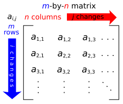
Matrices are a useful notion to encode linear maps. ^[45] They are written as a rectangular array of scalars as in the image at the right. Any m-by-n matrix ${\displaystyle A}$ gives rise to a linear map from Fⁿ to F^m, by the following $${\displaystyle \mathbf {x} =(x_{1},x_{2},\ldots ,x_{n})\mapsto \left(\sum _{j=1}^{n}a_{1j}x_{j},\sum _{j=1}^{n}a_{2j}x_{j},\ldots ,\sum _{j=1}^{n}a_{mj}x_{j}\right),}$$ where ${\textstyle \sum }$ denotes summation, or by using the matrix multiplication of the matrix ${\displaystyle A}$ with the coordinate vector ${\displaystyle \mathbf {x} }$:

$${\displaystyle \mathbf {x} \mapsto A\mathbf {x} .}$$

Moreover, after choosing bases of V and W, any linear map f : V → W is uniquely represented by a matrix via this assignment. ^[46]

The volume of this parallelepiped is the absolute value of the determinant of the 3-by-3 matrix formed by the vectors r₁, r₂, and r₃.

The determinant det (A) of a square matrix A is a scalar that tells whether the associated map is an isomorphism or not: to be so it is sufficient and necessary that the determinant is nonzero. ^[47] The linear transformation of Rⁿ corresponding to a real n-by-n matrix is orientation preserving if and only if its determinant is positive.

Eigenvalues and eigenvectors

Main article: Eigenvalues and eigenvectors

Endomorphisms, linear maps f : V → V, are particularly important since in this case vectors v can be compared with their image under f, f(v). Any nonzero vector v satisfying λv = f(v), where λ is a scalar, is called an eigenvector of f with eigenvalueλ. ^[48] Equivalently, v is an element of the kernel of the difference f − λ · Id (where Id is the identity map V → V). If V is finite-dimensional, this can be rephrased using determinants: f having eigenvalue λ is equivalent to $${\displaystyle \det(f-\lambda \cdot \operatorname {Id} )=0.}$$ By spelling out the definition of the determinant, the expression on the left hand side can be seen to be a polynomial function in λ, called the characteristic polynomial of f. ^[49] If the field F is large enough to contain a zero of this polynomial (which automatically happens for F algebraically closed, such as F = C) any linear map has at least one eigenvector. The vector space V may or may not possess an eigenbasis, a basis consisting of eigenvectors. This phenomenon is governed by the Jordan canonical form of the map. ^[50] The set of all eigenvectors corresponding to a particular eigenvalue of f forms a vector space known as the eigenspace corresponding to the eigenvalue (and f) in question.

Basic constructions

In addition to the above concrete examples, there are a number of standard linear algebraic constructions that yield vector spaces related to given ones.

Subspaces and quotient spaces

Main articles: Linear subspace and Quotient vector space

A line passing through the origin (blue, thick) in R is a linear subspace. It is the intersection of two planes (green and yellow).

A nonempty subset ${\displaystyle W}$ of a vector space ${\displaystyle V}$ that is closed under addition and scalar multiplication (and therefore contains the ${\displaystyle \mathbf {0} }$-vector of ${\displaystyle V}$) is called a linear subspace of ${\displaystyle V}$, or simply a subspace of ${\displaystyle V}$, when the ambient space is unambiguously a vector space. ^{[51] [nb 4]} Subspaces of ${\displaystyle V}$ are vector spaces (over the same field) in their own right. The intersection of all subspaces containing a given set ${\displaystyle S}$ of vectors is called its span, and it is the smallest subspace of ${\displaystyle V}$ containing the set ${\displaystyle S}$. Expressed in terms of elements, the span is the subspace consisting of all the linear combinations of elements of ${\displaystyle S}$. ^[52]

Linear subspace of dimension 1 and 2 are referred to as a line (also vector line), and a plane respectively. If W is an n-dimensional vector space, any subspace of dimension 1 less, i.e., of dimension ${\displaystyle n-1}$ is called a hyperplane . ^[53]

The counterpart to subspaces are quotient vector spaces. ^[54] Given any subspace ${\displaystyle W\subseteq V}$, the quotient space ${\displaystyle V/W}$ ("${\displaystyle V}$ modulo ${\displaystyle W}$") is defined as follows: as a set, it consists of $${\displaystyle \mathbf {v} +W=\{\mathbf {v} +\mathbf {w}$$ :\mathbf {w} \in W\},} where ${\displaystyle \mathbf {v} }$ is an arbitrary vector in ${\displaystyle V}$. The sum of two such elements ${\displaystyle \mathbf {v} _{1}+W}$ and ${\displaystyle \mathbf {v} _{2}+W}$ is ${\displaystyle \left(\mathbf {v} _{1}+\mathbf {v} _{2}\right)+W}$, and scalar multiplication is given by ${\displaystyle a\cdot (\mathbf {v} +W)=(a\cdot \mathbf {v} )+W}$. The key point in this definition is that ${\displaystyle \mathbf {v} _{1}+W=\mathbf {v} _{2}+W}$ if and only if the difference of ${\displaystyle \mathbf {v} _{1}}$ and ${\displaystyle \mathbf {v} _{2}}$ lies in ${\displaystyle W}$. ^{[nb 5]} This way, the quotient space "forgets" information that is contained in the subspace ${\displaystyle W}$.

The kernel ${\displaystyle \ker(f)}$ of a linear map ${\displaystyle f:V\to W}$ consists of vectors ${\displaystyle \mathbf {v} }$ that are mapped to ${\displaystyle \mathbf {0} }$ in ${\displaystyle W}$. ^[55] The kernel and the image ${\displaystyle \operatorname {im} (f)=\{f(\mathbf {v} ):\mathbf {v} \in V\}}$ are subspaces of ${\displaystyle V}$ and ${\displaystyle W}$, respectively. ^[56]

An important example is the kernel of a linear map ${\displaystyle \mathbf {x} \mapsto A\mathbf {x} }$ for some fixed matrix ${\displaystyle A}$. The kernel of this map is the subspace of vectors ${\displaystyle \mathbf {x} }$ such that ${\displaystyle A\mathbf {x} =\mathbf {0} }$, which is precisely the set of solutions to the system of homogeneous linear equations belonging to ${\displaystyle A}$. This concept also extends to linear differential equations $${\displaystyle a_{0}f+a_{1}{\frac {df}{dx}}+a_{2}{\frac {d^{2}f}{dx^{2}}}+\cdots +a_{n}{\frac {d^{n}f}{dx^{n}}}=0,}$$ where the coefficients ${\displaystyle a_{i}}$ are functions in ${\displaystyle x,}$ too. In the corresponding map $${\displaystyle f\mapsto D(f)=\sum _{i=0}^{n}a_{i}{\frac {d^{i}f}{dx^{i}}},}$$ the derivatives of the function ${\displaystyle f}$ appear linearly (as opposed to ${\displaystyle f^{\prime \prime }(x)^{2}}$, for example). Since differentiation is a linear procedure (that is, ${\displaystyle (f+g)^{\prime }=f^{\prime }+g^{\prime }}$ and ${\displaystyle (c\cdot f)^{\prime }=c\cdot f^{\prime }}$ for a constant ${\displaystyle c}$) this assignment is linear, called a linear differential operator. In particular, the solutions to the differential equation ${\displaystyle D(f)=0}$ form a vector space (over R or C). ^[57]

The existence of kernels and images is part of the statement that the category of vector spaces (over a fixed field ${\displaystyle F}$) is an abelian category, that is, a corpus of mathematical objects and structure-preserving maps between them (a category) that behaves much like the category of abelian groups. ^[58] Because of this, many statements such as the first isomorphism theorem (also called rank–nullity theorem in matrix-related terms) $${\displaystyle V/\ker(f)\;\equiv \;\operatorname {im} (f)}$$ and the second and third isomorphism theorem can be formulated and proven in a way very similar to the corresponding statements for groups.

Direct product and direct sum

Main articles: Direct product and Direct sum of modules

The direct product of vector spaces and the direct sum of vector spaces are two ways of combining an indexed family of vector spaces into a new vector space.

The direct product${\displaystyle \textstyle {\prod _{i\in I}V_{i}}}$ of a family of vector spaces ${\displaystyle V_{i}}$ consists of the set of all tuples ${\displaystyle \left(\mathbf {v} _{i}\right)_{i\in I}}$, which specify for each index ${\displaystyle i}$ in some index set ${\displaystyle I}$ an element ${\displaystyle \mathbf {v} _{i}}$ of ${\displaystyle V_{i}}$. ^[59] Addition and scalar multiplication is performed componentwise. A variant of this construction is the direct sum${\textstyle \bigoplus _{i\in I}V_{i}}$ (also called coproduct and denoted ${\textstyle \coprod _{i\in I}V_{i}}$), where only tuples with finitely many nonzero vectors are allowed. If the index set ${\displaystyle I}$ is finite, the two constructions agree, but in general they are different.

Tensor product

Main article: Tensor product of vector spaces

The tensor product${\displaystyle V\otimes _{F}W,}$ or simply ${\displaystyle V\otimes W,}$ of two vector spaces ${\displaystyle V}$ and ${\displaystyle W}$ is one of the central notions of multilinear algebra which deals with extending notions such as linear maps to several variables. A map ${\displaystyle g:V\times W\to X}$ from the Cartesian product ${\displaystyle V\times W}$ is called bilinear if ${\displaystyle g}$ is linear in both variables ${\displaystyle \mathbf {v} }$ and ${\displaystyle \mathbf {w} .}$ That is to say, for fixed ${\displaystyle \mathbf {w} }$ the map ${\displaystyle \mathbf {v} \mapsto g(\mathbf {v} ,\mathbf {w} )}$ is linear in the sense above and likewise for fixed ${\displaystyle \mathbf {v} .}$

Commutative diagram depicting the universal property of the tensor product

The tensor product is a particular vector space that is a universal recipient of bilinear maps ${\displaystyle g,}$ as follows. It is defined as the vector space consisting of finite (formal) sums of symbols called tensors $${\displaystyle \mathbf {v} _{1}\otimes \mathbf {w} _{1}+\mathbf {v} _{2}\otimes \mathbf {w} _{2}+\cdots +\mathbf {v} _{n}\otimes \mathbf {w} _{n},}$$ subject to the rules ^[60] $${\displaystyle {\begin{alignedat}{6}a\cdot (\mathbf {v} \otimes \mathbf {w} )~&=~(a\cdot \mathbf {v} )\otimes \mathbf {w} ~=~\mathbf {v} \otimes (a\cdot \mathbf {w} ),&&~~{\text{ where }}a{\text{ is a scalar}}\\(\mathbf {v} _{1}+\mathbf {v} _{2})\otimes \mathbf {w} ~&=~\mathbf {v} _{1}\otimes \mathbf {w} +\mathbf {v} _{2}\otimes \mathbf {w} &&\\\mathbf {v} \otimes (\mathbf {w} _{1}+\mathbf {w} _{2})~&=~\mathbf {v} \otimes \mathbf {w} _{1}+\mathbf {v} \otimes \mathbf {w} _{2}.&&\\\end{alignedat}}}$$ These rules ensure that the map ${\displaystyle f}$ from the ${\displaystyle V\times W}$ to ${\displaystyle V\otimes W}$ that maps a tuple ${\displaystyle (\mathbf {v} ,\mathbf {w} )}$ to ${\displaystyle \mathbf {v} \otimes \mathbf {w} }$ is bilinear. The universality states that given any vector space ${\displaystyle X}$ and any bilinear map ${\displaystyle g:V\times W\to X,}$ there exists a unique map ${\displaystyle u,}$ shown in the diagram with a dotted arrow, whose composition with ${\displaystyle f}$ equals ${\displaystyle g:}$${\displaystyle u(\mathbf {v} \otimes \mathbf {w} )=g(\mathbf {v} ,\mathbf {w} ).}$ ^[61] This is called the universal property of the tensor product, an instance of the method—much used in advanced abstract algebra—to indirectly define objects by specifying maps from or to this object.

Vector spaces with additional structure

From the point of view of linear algebra, vector spaces are completely understood insofar as any vector space over a given field is characterized, up to isomorphism, by its dimension. However, vector spaces per se do not offer a framework to deal with the question—crucial to analysis—whether a sequence of functions converges to another function. Likewise, linear algebra is not adapted to deal with infinite series, since the addition operation allows only finitely many terms to be added. Therefore, the needs of functional analysis require considering additional structures. ^[62]

A vector space may be given a partial order ${\displaystyle \,\leq ,\,}$ under which some vectors can be compared. ^[63] For example, ${\displaystyle n}$-dimensional real space ${\displaystyle \mathbf {R} ^{n}}$ can be ordered by comparing its vectors componentwise. Ordered vector spaces, for example Riesz spaces, are fundamental to Lebesgue integration, which relies on the ability to express a function as a difference of two positive functions $${\displaystyle f=f^{+}-f^{-}.}$$ where ${\displaystyle f^{+}}$ denotes the positive part of ${\displaystyle f}$ and ${\displaystyle f^{-}}$ the negative part. ^[64]

Normed vector spaces and inner product spaces

Main articles: Normed vector space and Inner product space

"Measuring" vectors is done by specifying a norm, a datum which measures lengths of vectors, or by an inner product, which measures angles between vectors. Norms and inner products are denoted ${\displaystyle |\mathbf {v} |}$ and ${\displaystyle \langle \mathbf {v} ,\mathbf {w} \rangle ,}$ respectively. The datum of an inner product entails that lengths of vectors can be defined too, by defining the associated norm ${\textstyle |\mathbf {v} |:={\sqrt {\langle \mathbf {v} ,\mathbf {v} \rangle }}.}$ Vector spaces endowed with such data are known as normed vector spaces and inner product spaces, respectively. ^[65]

Coordinate space ${\displaystyle F^{n}}$ can be equipped with the standard dot product: $${\displaystyle \langle \mathbf {x} ,\mathbf {y} \rangle =\mathbf {x} \cdot \mathbf {y} =x_{1}y_{1}+\cdots +x_{n}y_{n}.}$$ In ${\displaystyle \mathbf {R} ^{2},}$ this reflects the common notion of the angle between two vectors ${\displaystyle \mathbf {x} }$ and ${\displaystyle \mathbf {y} ,}$ by the law of cosines: $${\displaystyle \mathbf {x} \cdot \mathbf {y} =\cos \left(\angle (\mathbf {x} ,\mathbf {y} )\right)\cdot |\mathbf {x} |\cdot |\mathbf {y} |.}$$ Because of this, two vectors satisfying ${\displaystyle \langle \mathbf {x} ,\mathbf {y} \rangle =0}$ are called orthogonal. An important variant of the standard dot product is used in Minkowski space: ${\displaystyle \mathbf {R} ^{4}}$ endowed with the Lorentz product ^[66] $${\displaystyle \langle \mathbf {x} |\mathbf {y} \rangle =x_{1}y_{1}+x_{2}y_{2}+x_{3}y_{3}-x_{4}y_{4}.}$$ In contrast to the standard dot product, it is not positive definite: ${\displaystyle \langle \mathbf {x} |\mathbf {x} \rangle }$ also takes negative values, for example, for ${\displaystyle \mathbf {x} =(0,0,0,1).}$ Singling out the fourth coordinate—corresponding to time, as opposed to three space-dimensions—makes it useful for the mathematical treatment of special relativity. Note that in other conventions time is often written as the first, or "zeroeth" component so that the Lorentz product is written $${\displaystyle \langle \mathbf {x} |\mathbf {y} \rangle =-x_{0}y_{0}+x_{1}y_{1}+x_{2}y_{2}+x_{3}y_{3}.}$$

Topological vector spaces

Main article: Topological vector space

Convergence questions are treated by considering vector spaces ${\displaystyle V}$ carrying a compatible topology, a structure that allows one to talk about elements being close to each other. ^[67] Compatible here means that addition and scalar multiplication have to be continuous maps. Roughly, if ${\displaystyle \mathbf {x} }$ and ${\displaystyle \mathbf {y} }$ in ${\displaystyle V}$, and ${\displaystyle a}$ in ${\displaystyle F}$ vary by a bounded amount, then so do ${\displaystyle \mathbf {x} +\mathbf {y} }$ and ${\displaystyle a\mathbf {x} .}$ ^{[nb 6]} To make sense of specifying the amount a scalar changes, the field ${\displaystyle F}$ also has to carry a topology in this context; a common choice is the reals or the complex numbers.

In such topological vector spaces one can consider series of vectors. The infinite sum $${\displaystyle \sum _{i=1}^{\infty }f_{i}~=~\lim _{n\to \infty }f_{1}+\cdots +f_{n}}$$ denotes the limit of the corresponding finite partial sums of the sequence ${\displaystyle f_{1},f_{2},\ldots }$ of elements of ${\displaystyle V.}$ For example, the ${\displaystyle f_{i}}$ could be (real or complex) functions belonging to some function space ${\displaystyle V,}$ in which case the series is a function series. The mode of convergence of the series depends on the topology imposed on the function space. In such cases, pointwise convergence and uniform convergence are two prominent examples. ^[68]

Unit "spheres" in ${\displaystyle \mathbf {R} ^{2}}$ consist of plane vectors of norm 1. Depicted are the unit spheres in different ${\displaystyle p}$-norms, for ${\displaystyle p=1,2,}$ and ${\displaystyle \infty .}$ The bigger diamond depicts points of 1-norm equal to 2.

A way to ensure the existence of limits of certain infinite series is to restrict attention to spaces where any Cauchy sequence has a limit; such a vector space is called complete. Roughly, a vector space is complete provided that it contains all necessary limits. For example, the vector space of polynomials on the unit interval ${\displaystyle [0,1],}$ equipped with the topology of uniform convergence is not complete because any continuous function on ${\displaystyle [0,1]}$ can be uniformly approximated by a sequence of polynomials, by the Weierstrass approximation theorem. ^[69] In contrast, the space of all continuous functions on ${\displaystyle [0,1]}$ with the same topology is complete. ^[70] A norm gives rise to a topology by defining that a sequence of vectors ${\displaystyle \mathbf {v} _{n}}$ converges to ${\displaystyle \mathbf {v} }$ if and only if $${\displaystyle \lim _{n\to \infty }|\mathbf {v} _{n}-\mathbf {v} |=0.}$$ Banach and Hilbert spaces are complete topological vector spaces whose topologies are given, respectively, by a norm and an inner product. Their study—a key piece of functional analysis—focuses on infinite-dimensional vector spaces, since all norms on finite-dimensional topological vector spaces give rise to the same notion of convergence. ^[71] The image at the right shows the equivalence of the ${\displaystyle 1}$-norm and ${\displaystyle \infty }$-norm on ${\displaystyle \mathbf {R} ^{2}:}$ as the unit "balls" enclose each other, a sequence converges to zero in one norm if and only if it so does in the other norm. In the infinite-dimensional case, however, there will generally be inequivalent topologies, which makes the study of topological vector spaces richer than that of vector spaces without additional data.

From a conceptual point of view, all notions related to topological vector spaces should match the topology. For example, instead of considering all linear maps (also called functionals) ${\displaystyle V\to W,}$ maps between topological vector spaces are required to be continuous. ^[72] In particular, the (topological) dual space ${\displaystyle V^{*}}$ consists of continuous functionals ${\displaystyle V\to \mathbf {R} }$ (or to ${\displaystyle \mathbf {C} }$). The fundamental Hahn–Banach theorem is concerned with separating subspaces of appropriate topological vector spaces by continuous functionals. ^[73]

Banach spaces

Main article: Banach space

Banach spaces , introduced by Stefan Banach, are complete normed vector spaces. ^[74]

A first example is the vector space ${\displaystyle \ell ^{p}}$ consisting of infinite vectors with real entries ${\displaystyle \mathbf {x} =\left(x_{1},x_{2},\ldots ,x_{n},\ldots \right)}$ whose ${\displaystyle p}$-norm ${\displaystyle (1\leq p\leq \infty )}$ given by $${\displaystyle \|\mathbf {x} \|_{\infty }:=\sup _{i}|x_{i}|\qquad {\text{ for }}p=\infty ,{\text{ and }}}$$$${\displaystyle \|\mathbf {x} \|_{p}:=\left(\sum _{i}|x_{i}|^{p}\right)^{\frac {1}{p}}\qquad {\text{ for }}p<\infty .}$$

The topologies on the infinite-dimensional space ${\displaystyle \ell ^{p}}$ are inequivalent for different ${\displaystyle p.}$ For example, the sequence of vectors ${\displaystyle \mathbf {x} _{n}=\left(2^{-n},2^{-n},\ldots ,2^{-n},0,0,\ldots \right),}$ in which the first ${\displaystyle 2^{n}}$ components are ${\displaystyle 2^{-n}}$ and the following ones are ${\displaystyle 0,}$ converges to the zero vector for ${\displaystyle p=\infty ,}$ but does not for ${\displaystyle p=1:}$$${\displaystyle \|\mathbf {x} _{n}\|_{\infty }=\sup(2^{-n},0)=2^{-n}\to 0,}$$ but $${\displaystyle \|\mathbf {x} _{n}\|_{1}=\sum _{i=1}^{2^{n}}2^{-n}=2^{n}\cdot 2^{-n}=1.}$$

More generally than sequences of real numbers, functions ${\displaystyle f:\Omega \to \mathbb {R} }$ are endowed with a norm that replaces the above sum by the Lebesgue integral $${\displaystyle \|f\|_{p}:=\left(\int _{\Omega }|f(x)|^{p}\,{d\mu (x)}\right)^{\frac {1}{p}}.}$$

The space of integrable functions on a given domain ${\displaystyle \Omega }$ (for example an interval) satisfying ${\displaystyle \|f\|_{p}<\infty ,}$ and equipped with this norm are called Lebesgue spaces, denoted ${\displaystyle L^{\;\!p}(\Omega ).}$ ^{[nb 7]}

These spaces are complete. ^[75] (If one uses the Riemann integral instead, the space is not complete, which may be seen as a justification for Lebesgue's integration theory. ^{[nb 8]} ) Concretely this means that for any sequence of Lebesgue-integrable functions ${\displaystyle f_{1},f_{2},\ldots ,f_{n},\ldots }$ with ${\displaystyle \|f_{n}\|_{p}<\infty ,}$ satisfying the condition $${\displaystyle \lim _{k,\ n\to \infty }\int _{\Omega }\left|f_{k}(x)-f_{n}(x)\right|^{p}\,{d\mu (x)}=0}$$ there exists a function ${\displaystyle f(x)}$ belonging to the vector space ${\displaystyle L^{\;\!p}(\Omega )}$ such that $${\displaystyle \lim _{k\to \infty }\int _{\Omega }\left|f(x)-f_{k}(x)\right|^{p}\,{d\mu (x)}=0.}$$

Imposing boundedness conditions not only on the function, but also on its derivatives leads to Sobolev spaces. ^[76]

Hilbert spaces

Main article: Hilbert space

The succeeding snapshots show summation of 1 to 5 terms in approximating a periodic function (blue) by finite sum of sine functions (red).

Complete inner product spaces are known as Hilbert spaces, in honor of David Hilbert. ^[77] The Hilbert space ${\displaystyle L^{2}(\Omega ),}$ with inner product given by $${\displaystyle \langle f\ ,\ g\rangle =\int _{\Omega }f(x){\overline {g(x)}}\,dx,}$$ where ${\displaystyle {\overline {g(x)}}}$ denotes the complex conjugate of ${\displaystyle g(x),}$ ^{[78] [nb 9]} is a key case.

By definition, in a Hilbert space, any Cauchy sequence converges to a limit. Conversely, finding a sequence of functions ${\displaystyle f_{n}}$ with desirable properties that approximate a given limit function is equally crucial. Early analysis, in the guise of the Taylor approximation, established an approximation of differentiable functions ${\displaystyle f}$ by polynomials. ^[79] By the Stone–Weierstrass theorem, every continuous function on ${\displaystyle [a,b]}$ can be approximated as closely as desired by a polynomial. ^[80] A similar approximation technique by trigonometric functions is commonly called Fourier expansion, and is much applied in engineering. More generally, and more conceptually, the theorem yields a simple description of what "basic functions", or, in abstract Hilbert spaces, what basic vectors suffice to generate a Hilbert space ${\displaystyle H,}$ in the sense that the closure of their span (that is, finite linear combinations and limits of those) is the whole space. Such a set of functions is called a basis of ${\displaystyle H,}$ its cardinality is known as the Hilbert space dimension. ^{[nb 10]} Not only does the theorem exhibit suitable basis functions as sufficient for approximation purposes, but also together with the Gram–Schmidt process, it enables one to construct a basis of orthogonal vectors. ^[81] Such orthogonal bases are the Hilbert space generalization of the coordinate axes in finite-dimensional Euclidean space.

The solutions to various differential equations can be interpreted in terms of Hilbert spaces. For example, a great many fields in physics and engineering lead to such equations, and frequently solutions with particular physical properties are used as basis functions, often orthogonal. ^[82] As an example from physics, the time-dependent Schrödinger equation in quantum mechanics describes the change of physical properties in time by means of a partial differential equation, whose solutions are called wavefunctions. ^[83] Definite values for physical properties such as energy, or momentum, correspond to eigenvalues of a certain (linear) differential operator and the associated wavefunctions are called eigenstates. The spectral theorem decomposes a linear compact operator acting on functions in terms of these eigenfunctions and their eigenvalues. ^[84]

Algebras over fields

Main articles: Algebra over a field and Lie algebra

A hyperbola, given by the equation ${\displaystyle x\cdot y=1.}$ The coordinate ring of functions on this hyperbola is given by ${\displaystyle \mathbf {R} [x,y]/(x\cdot y-1),}$ an infinite-dimensional vector space over ${\displaystyle \mathbf {R} .}$

General vector spaces do not possess a multiplication between vectors. A vector space equipped with an additional bilinear operator defining the multiplication of two vectors is an algebra over a field (or F-algebra if the field F is specified). ^[85]

For example, the set of all polynomials ${\displaystyle p(t)}$ forms an algebra known as the polynomial ring: using that the sum of two polynomials is a polynomial, they form a vector space; they form an algebra since the product of two polynomials is again a polynomial. Rings of polynomials (in several variables) and their quotients form the basis of algebraic geometry, because they are rings of functions of algebraic geometric objects. ^[86]

Another crucial example are Lie algebras , which are neither commutative nor associative, but the failure to be so is limited by the constraints (${\displaystyle [x,y]}$ denotes the product of ${\displaystyle x}$ and ${\displaystyle y}$):

• ${\displaystyle [x,y]=-[y,x]}$ (anticommutativity), and
• ${\displaystyle [x,[y,z]]+[y,[z,x]]+[z,[x,y]]=0}$ (Jacobi identity). ^[87]

Examples include the vector space of ${\displaystyle n}$-by-${\displaystyle n}$ matrices, with ${\displaystyle [x,y]=xy-yx,}$ the commutator of two matrices, and ${\displaystyle \mathbf {R} ^{3},}$ endowed with the cross product.

The tensor algebra ${\displaystyle \operatorname {T} (V)}$ is a formal way of adding products to any vector space ${\displaystyle V}$ to obtain an algebra. ^[88] As a vector space, it is spanned by symbols, called simple tensors $${\displaystyle \mathbf {v} _{1}\otimes \mathbf {v} _{2}\otimes \cdots \otimes \mathbf {v} _{n},}$$ where the degree ${\displaystyle n}$ varies. The multiplication is given by concatenating such symbols, imposing the distributive law under addition, and requiring that scalar multiplication commute with the tensor product ⊗, much the same way as with the tensor product of two vector spaces introduced in the above section on tensor products. In general, there are no relations between ${\displaystyle \mathbf {v} _{1}\otimes \mathbf {v} _{2}}$ and ${\displaystyle \mathbf {v} _{2}\otimes \mathbf {v} _{1}.}$ Forcing two such elements to be equal leads to the symmetric algebra, whereas forcing ${\displaystyle \mathbf {v} _{1}\otimes \mathbf {v} _{2}=-\mathbf {v} _{2}\otimes \mathbf {v} _{1}}$ yields the exterior algebra. ^[89]

Related structures

Vector bundles

Main articles: Vector bundle and Tangent bundle

A Möbius strip. Locally, it looks like U × R.

A vector bundle is a family of vector spaces parametrized continuously by a topological space X. ^[90] More precisely, a vector bundle over X is a topological space E equipped with a continuous map $${\displaystyle \pi :E\to X}$$ such that for every x in X, the fiber π⁻¹(x) is a vector space. The case dim V = 1 is called a line bundle. For any vector space V, the projection X × V → X makes the product X × V into a "trivial" vector bundle. Vector bundles over X are required to be locally a product of X and some (fixed) vector space V: for every x in X, there is a neighborhood U of x such that the restriction of π to π⁻¹(U) is isomorphic ^{[nb 11]} to the trivial bundle U × V → U. Despite their locally trivial character, vector bundles may (depending on the shape of the underlying space X) be "twisted" in the large (that is, the bundle need not be (globally isomorphic to) the trivial bundle X × V). For example, the Möbius strip can be seen as a line bundle over the circle S¹ (by identifying open intervals with the real line). It is, however, different from the cylinder S¹ × R, because the latter is orientable whereas the former is not. ^[91]

Properties of certain vector bundles provide information about the underlying topological space. For example, the tangent bundle consists of the collection of tangent spaces parametrized by the points of a differentiable manifold. The tangent bundle of the circle S¹ is globally isomorphic to S¹ × R, since there is a global nonzero vector field on S¹. ^{[nb 12]} In contrast, by the hairy ball theorem, there is no (tangent) vector field on the 2-sphere S² which is everywhere nonzero. ^[92] K-theory studies the isomorphism classes of all vector bundles over some topological space. ^[93] In addition to deepening topological and geometrical insight, it has purely algebraic consequences, such as the classification of finite-dimensional real division algebras: R, C, the quaternions H and the octonions O.

The cotangent bundle of a differentiable manifold consists, at every point of the manifold, of the dual of the tangent space, the cotangent space. Sections of that bundle are known as differential one-forms.

Modules

Main article: Module

Modules are to rings what vector spaces are to fields: the same axioms, applied to a ring R instead of a field F, yield modules. ^[94] The theory of modules, compared to that of vector spaces, is complicated by the presence of ring elements that do not have multiplicative inverses. For example, modules need not have bases, as the Z-module (that is, abelian group) Z/2Z shows; those modules that do (including all vector spaces) are known as free modules. Nevertheless, a vector space can be compactly defined as a module over a ring which is a field, with the elements being called vectors. Some authors use the term vector space to mean modules over a division ring. ^[95] The algebro-geometric interpretation of commutative rings via their spectrum allows the development of concepts such as locally free modules, the algebraic counterpart to vector bundles.

Affine and projective spaces

Main articles: Affine space and Projective space

An affine plane (light blue) in R . It is a two-dimensional subspace shifted by a vector x (red).

Roughly, affine spaces are vector spaces whose origins are not specified. ^[96] More precisely, an affine space is a set with a free transitive vector space action. In particular, a vector space is an affine space over itself, by the map $${\displaystyle V\times V\to W,\;(\mathbf {v} ,\mathbf {a} )\mapsto \mathbf {a} +\mathbf {v} .}$$ If W is a vector space, then an affine subspace is a subset of W obtained by translating a linear subspace V by a fixed vector x ∈ W; this space is denoted by x + V (it is a coset of V in W) and consists of all vectors of the form x + v for v ∈ V. An important example is the space of solutions of a system of inhomogeneous linear equations $${\displaystyle A\mathbf {v} =\mathbf {b} }$$ generalizing the homogeneous case discussed in the above section on linear equations, which can be found by setting ${\displaystyle \mathbf {b} =\mathbf {0} }$ in this equation. ^[97] The space of solutions is the affine subspace x + V where x is a particular solution of the equation, and V is the space of solutions of the homogeneous equation (the nullspace of A).

The set of one-dimensional subspaces of a fixed finite-dimensional vector space V is known as projective space; it may be used to formalize the idea of parallel lines intersecting at infinity. ^[98] Grassmannians and flag manifolds generalize this by parametrizing linear subspaces of fixed dimension k and flags of subspaces, respectively.

Notes

1. It is also common, especially in physics, to denote vectors with an arrow on top: ${\displaystyle {\vec {v}}.}$ It is also common, especially in higher mathematics, to not use any typographical method for distinguishing vectors from other mathematical objects.
2. Scalar multiplication is not to be confused with the scalar product, which is an additional operation on some specific vector spaces, called inner product spaces. Scalar multiplication is the multiplication of a vector by a scalar that produces a vector, while the scalar product is a multiplication of two vectors that produces a scalar.
3. This axiom is not an associative property, since it refers to two different operations, scalar multiplication and field multiplication. So, it is independent from the associativity of field multiplication, which is assumed by field axioms.
4. This is typically the case when a vector space is also considered as an affine space. In this case, a linear subspace contains the zero vector, while an affine subspace does not necessarily contain it.
5. Some authors, such as Roman (2005), choose to start with this equivalence relation and derive the concrete shape of ${\displaystyle V/W}$ from this.
6. This requirement implies that the topology gives rise to a uniform structure, Bourbaki (1989), loc = ch. II.
7. The triangle inequality for ${\displaystyle \|f+g\|_{p}\leq \|f\|_{p}+\|g\|_{p}}$ is provided by the Minkowski inequality. For technical reasons, in the context of functions one has to identify functions that agree almost everywhere to get a norm, and not only a seminorm.
8. "Many functions in ${\displaystyle L^{2}}$ of Lebesgue measure, being unbounded, cannot be integrated with the classical Riemann integral. So spaces of Riemann integrable functions would not be complete in the ${\displaystyle L^{2}}$ norm, and the orthogonal decomposition would not apply to them. This shows one of the advantages of Lebesgue integration.", Dudley (1989), §5.3, p. 125.
9. For ${\displaystyle p\neq 2,}$${\displaystyle L^{p}(\Omega )}$ is not a Hilbert space.
10. A basis of a Hilbert space is not the same thing as a basis of a linear algebra. For distinction, a linear algebra basis for a Hilbert space is called a Hamel basis.
11. That is, there is a homeomorphism from π⁻¹(U) to V × U which restricts to linear isomorphisms between fibers.
12. A line bundle, such as the tangent bundle of S¹ is trivial if and only if there is a section that vanishes nowhere, see Husemoller (1994), Corollary 8.3. The sections of the tangent bundle are just vector fields.

Citations

1. Lang 2002.
2. Brown 1991, p. 86.
3. Roman 2005, ch. 1, p. 27.
4. Brown 1991, p. 87.
5. Springer 2000, p.  185; Brown 1991, p. 86.
6. Atiyah & Macdonald 1969, p. 17.
7. Bourbaki 1998, §1.1, Definition 2.
8. Brown 1991, p. 94.
9. Brown 1991, pp. 99–101.
10. Brown 1991, p. 92.
11. Stoll & Wong 1968, p.  14.
12. Roman 2005, pp. 41–42.
13. Lang 1987, p. 10–11; Anton & Rorres 2010, p.  212.
14. Blass 1984.
15. Joshi 1989, p.  450.
16. Heil 2011, p.  126.
17. Halmos 1948, p.  12.
18. Bourbaki 1969, ch. "Algèbre linéaire et algèbre multilinéaire", pp. 78–91.
19. Bolzano 1804.
20. Möbius 1827.
21. Bellavitis 1833.
22. Dorier 1995.
23. Hamilton 1853.
24. Grassmann 2000.
25. Peano 1888, ch. IX.
26. Guo 2021.
27. Moore 1995, pp. 268–271.
28. Banach 1922.
29. Dorier 1995; Moore 1995.
30. Kreyszig 2020, p.  355.
31. Kreyszig 2020, p.  358–359.
32. Jain 2001, p.  11.
33. Lang 1987, ch. I.1.
34. Lang 2002, ch. V.1.
35. Lang 1993, ch. XII.3., p. 335.
36. Lang 1987, ch. VI.3..
37. Roman 2005, ch. 2, p. 45.
38. Lang 1987, ch. IV.4, Corollary, p. 106.
39. Nicholson 2018, ch. 7.3.
40. Lang 1987, Example IV.2.6.
41. Lang 1987, ch. VI.6.
42. Halmos 1974, p. 28, Ex. 9.
43. Lang 1987, Theorem IV.2.1, p. 95.
44. Roman 2005, Th. 2.5 and 2.6, p. 49.
45. Lang 1987, ch. V.1.
46. Lang 1987, ch. V.3., Corollary, p. 106.
47. Lang 1987, Theorem VII.9.8, p. 198.
48. Roman 2005, ch. 8, p. 135–156.
49. & Lang 1987, ch. IX.4.
50. Roman 2005, ch. 8, p. 140.
51. Roman 2005, ch. 1, p. 29.
52. Roman 2005, ch. 1, p. 35.
53. Nicholson 2018, ch. 10.4.
54. Roman 2005, ch. 3, p. 64.
55. Lang 1987, ch. IV.3..
56. Roman 2005, ch. 2, p. 48.
57. Nicholson 2018, ch. 7.4.
58. Mac Lane 1998.
59. Roman 2005, ch. 1, pp. 31–32.
60. Lang 2002, ch. XVI.1.
61. Roman (2005), Th. 14.3. See also Yoneda lemma.
62. Rudin 1991, p.3.
63. Schaefer & Wolff 1999, pp. 204–205.
64. Bourbaki 2004, ch. 2, p. 48.
65. Roman 2005, ch. 9.
66. Naber 2003, ch. 1.2.
67. Treves 1967; Bourbaki 1987.
68. Schaefer & Wolff 1999, p. 7.
69. Kreyszig 1989 , §4.11-5
70. Kreyszig 1989 , §1.5-5
71. Choquet 1966, Proposition III.7.2.
72. Treves 1967, p. 34–36.
73. Lang 1983, Cor. 4.1.2, p. 69.
74. Treves 1967, ch. 11.
75. Treves 1967, Theorem 11.2, p. 102.
76. Evans 1998, ch. 5.
77. Treves 1967, ch. 12.
78. Dennery & Krzywicki 1996, p.190.
79. Lang 1993, Th. XIII.6, p. 349.
80. Lang 1993, Th. III.1.1.
81. Choquet 1966, Lemma III.16.11.
82. Kreyszig 1999, Chapter 11.
83. Griffiths 1995, Chapter 1.
84. Lang 1993, ch. XVII.3.
85. Lang 2002, ch. III.1, p. 121.
86. Eisenbud 1995, ch. 1.6.
87. Varadarajan 1974.
88. Lang 2002, ch. XVI.7.
89. Lang 2002, ch. XVI.8.
90. Spivak 1999, ch. 3.
91. Kreyszig 1991, §34, p. 108.
92. Eisenberg & Guy 1979.
93. Atiyah 1989.
94. Artin 1991, ch. 12.
95. Grillet 2007.
96. Meyer 2000, Example 5.13.5, p. 436.
97. Meyer 2000, Exercise 5.13.15–17, p. 442.
98. Coxeter 1987.

References

Algebra

• Anton, Howard; Rorres, Chris (2010), Elementary Linear Algebra: Applications Version (10th ed.), John Wiley & Sons
• Artin, Michael (1991), Algebra, Prentice Hall, ISBN   978-0-89871-510-1
• Brown, William A. (1991), Matrices and vector spaces , New York: M. Dekker, ISBN   978-0-8247-8419-5
• Grillet, Pierre Antoine (2007), Abstract algebra, vol. 242, Springer Science & Business Media, doi:10.1007/978-0-387-71568-1, ISBN   978-0-387-71568-1
• Halmos, Paul R. (1948), Finite Dimensional Vector Spaces, vol. 7, Princeton University Press
• Heil, Christopher (2011), A Basis Theory Primer: Expanded Edition, Applied and Numerical Harmonic Analysis, Birkhäuser, doi:10.1007/978-0-8176-4687-5, ISBN   978-0-8176-4687-5
• Jain, M. C. (2001), Vector Spaces and Matrices in Physics, CRC Press, ISBN   978-0-8493-0978-6
• Joshi, K. D. (1989), Foundations of Discrete Mathematics, John Wiley & Sons
• Kreyszig, Erwin (2020), Advanced Engineering Mathematics, John Wiley & Sons, ISBN   978-1-119-45592-9
• Lang, Serge (1987), Linear algebra, Undergraduate Texts in Mathematics (3rd ed.), Springer, doi:10.1007/978-1-4757-1949-9, ISBN   978-1-4757-1949-9
• Lang, Serge (2002), Algebra, Graduate Texts in Mathematics, vol. 211 (Revised third ed.), New York: Springer-Verlag, ISBN   978-0-387-95385-4, MR   1878556
• Mac Lane, Saunders (1999), Algebra (3rd ed.), American Mathematical Soc., pp. 193–222, ISBN   978-0-8218-1646-2
• Meyer, Carl D. (2000), Matrix Analysis and Applied Linear Algebra, SIAM, ISBN   978-0-89871-454-8
• Nicholson, W. Keith (2018), Linear Algebra with Applications, Lyryx
• Roman, Steven (2005), Advanced Linear Algebra, Graduate Texts in Mathematics, vol. 135 (2nd ed.), Berlin, New York: Springer-Verlag, ISBN   978-0-387-24766-3
• Spindler, Karlheinz (1993), Abstract Algebra with Applications: Volume 1: Vector spaces and groups, CRC, ISBN   978-0-8247-9144-5
• Springer, T.A. (2000), Linear Algebraic Groups, Springer, ISBN   978-0-8176-4840-4
• Stoll, R. R.; Wong, E. T. (1968), Linear Algebra, Academic Press
• van der Waerden, Bartel Leendert (1993), Algebra (in German) (9th ed.), Berlin, New York: Springer-Verlag, ISBN   978-3-540-56799-8

Analysis

• Bourbaki, Nicolas (1987), Topological vector spaces, Elements of mathematics, Berlin, New York: Springer-Verlag, ISBN   978-3-540-13627-9
• Bourbaki, Nicolas (2004), Integration I, Berlin, New York: Springer-Verlag, ISBN   978-3-540-41129-1
• Braun, Martin (1993), Differential equations and their applications: an introduction to applied mathematics, Berlin, New York: Springer-Verlag, ISBN   978-0-387-97894-9
• BSE-3 (2001) [1994], "Tangent plane", Encyclopedia of Mathematics , EMS Press
• Choquet, Gustave (1966), Topology, Boston, MA: Academic Press
• Dennery, Philippe; Krzywicki, Andre (1996), Mathematics for Physicists, Courier Dover Publications, ISBN   978-0-486-69193-0
• Dudley, Richard M. (1989), Real analysis and probability, The Wadsworth & Brooks/Cole Mathematics Series, Pacific Grove, CA: Wadsworth & Brooks/Cole Advanced Books & Software, ISBN   978-0-534-10050-6
• Dunham, William (2005), The Calculus Gallery, Princeton University Press, ISBN   978-0-691-09565-3
• Evans, Lawrence C. (1998), Partial differential equations, Providence, R.I.: American Mathematical Society, ISBN   978-0-8218-0772-9
• Folland, Gerald B. (1992), Fourier Analysis and Its Applications, Brooks-Cole, ISBN   978-0-534-17094-3
• Gasquet, Claude; Witomski, Patrick (1999), Fourier Analysis and Applications: Filtering, Numerical Computation, Wavelets, Texts in Applied Mathematics, New York: Springer-Verlag, ISBN   978-0-387-98485-8
• Ifeachor, Emmanuel C.; Jervis, Barrie W. (2001), Digital Signal Processing: A Practical Approach (2nd ed.), Harlow, Essex, England: Prentice-Hall (published 2002), ISBN   978-0-201-59619-9
• Krantz, Steven G. (1999), A Panorama of Harmonic Analysis, Carus Mathematical Monographs, Washington, DC: Mathematical Association of America, ISBN   978-0-88385-031-2
• Kreyszig, Erwin (1988), Advanced Engineering Mathematics (6th ed.), New York: John Wiley & Sons, ISBN   978-0-471-85824-9
• Kreyszig, Erwin (1989), Introductory functional analysis with applications, Wiley Classics Library, New York: John Wiley & Sons, ISBN   978-0-471-50459-7, MR   0992618
• Lang, Serge (1983), Real analysis, Addison-Wesley, ISBN   978-0-201-14179-5
• Lang, Serge (1993), Real and functional analysis, Berlin, New York: Springer-Verlag, ISBN   978-0-387-94001-4
• Loomis, Lynn H. (2011) [1953], An introduction to abstract harmonic analysis, Dover, hdl: 2027/uc1.b4250788 , ISBN   978-0-486-48123-4, OCLC   702357363
• Narici, Lawrence; Beckenstein, Edward (2011). Topological Vector Spaces. Pure and applied mathematics (Second ed.). Boca Raton, FL: CRC Press. ISBN   978-1584888666. OCLC   144216834.
• Rudin, Walter (1991), Functional analysis (2 ed.), McGraw-Hill, ISBN   0070542368
• Schaefer, Helmut H.; Wolff, Manfred P. (1999). Topological Vector Spaces. GTM. Vol. 8 (Second ed.). New York, NY: Springer New York Imprint Springer. ISBN   978-1-4612-7155-0. OCLC   840278135.
• Treves, François (1967), Topological vector spaces, distributions and kernels, Boston, MA: Academic Press

Historical references

• Banach, Stefan (1922), "Sur les opérations dans les ensembles abstraits et leur application aux équations intégrales (On operations in abstract sets and their application to integral equations)" (PDF), Fundamenta Mathematicae (in French), 3: 133–181, doi:10.4064/fm-3-1-133-181, ISSN   0016-2736
• Bolzano, Bernard (1804), Betrachtungen über einige Gegenstände der Elementargeometrie (Considerations of some aspects of elementary geometry) (in German)
• Bellavitis, Giuso (1833), "Sopra alcune applicazioni di un nuovo metodo di geometria analitica", Il poligrafo giornale di scienze, lettre ed arti, 13, Verona: 53–61.
• Bourbaki, Nicolas (1969), Éléments d'histoire des mathématiques (Elements of history of mathematics) (in French), Paris: Hermann
• Dorier, Jean-Luc (1995), "A general outline of the genesis of vector space theory", Historia Mathematica , 22 (3): 227–261, doi: 10.1006/hmat.1995.1024 , MR   1347828
• Fourier, Jean Baptiste Joseph (1822), Théorie analytique de la chaleur (in French), Chez Firmin Didot, père et fils
• Grassmann, Hermann (1844), Die Lineale Ausdehnungslehre - Ein neuer Zweig der Mathematik (in German), O. Wigand, reprint: Grassmann, Hermann (2000), Kannenberg, L.C. (ed.), Extension Theory, translated by Kannenberg, Lloyd C., Providence, R.I.: American Mathematical Society, ISBN   978-0-8218-2031-5
• Guo, Hongyu (2021-06-16), What Are Tensors Exactly?, World Scientific, ISBN   978-981-12-4103-1
• Hamilton, William Rowan (1853), Lectures on Quaternions, Royal Irish Academy
• Möbius, August Ferdinand (1827), Der Barycentrische Calcul : ein neues Hülfsmittel zur analytischen Behandlung der Geometrie (Barycentric calculus: a new utility for an analytic treatment of geometry) (in German), archived from the original on 2006-11-23
• Moore, Gregory H. (1995), "The axiomatization of linear algebra: 1875–1940", Historia Mathematica , 22 (3): 262–303, doi: 10.1006/hmat.1995.1025
• Peano, Giuseppe (1888), Calcolo Geometrico secondo l'Ausdehnungslehre di H. Grassmann preceduto dalle Operazioni della Logica Deduttiva (in Italian), Turin
• Peano, G. (1901) Formulario mathematico: vct axioms via Internet Archive

Further references

• Ashcroft, Neil; Mermin, N. David (1976), Solid State Physics , Toronto: Thomson Learning, ISBN   978-0-03-083993-1
• Atiyah, Michael Francis (1989), K-theory, Advanced Book Classics (2nd ed.), Addison-Wesley, ISBN   978-0-201-09394-0, MR   1043170
• Atiyah, Michael Francis; Macdonald, Ian Grant (1969), Introduction to Commutative Algebra, Advanced Book Classics, Addison-Wesley
• Blass, Andreas (1984), "Existence of bases implies the axiom of choice" (PDF), Axiomatic set theory, Contemporary Mathematics volume 31, Providence, R.I.: American Mathematical Society, pp. 31–33, ISBN   978-0-8218-5026-8, MR   0763890
• Bourbaki, Nicolas (1998), Elements of Mathematics : Algebra I Chapters 1-3, Berlin, New York: Springer-Verlag, ISBN   978-3-540-64243-5
• Bourbaki, Nicolas (1989), General Topology. Chapters 1-4, Berlin, New York: Springer-Verlag, ISBN   978-3-540-64241-1
• Coxeter, Harold Scott MacDonald (1987), Projective Geometry (2nd ed.), Berlin, New York: Springer-Verlag, ISBN   978-0-387-96532-1
• Eisenberg, Murray; Guy, Robert (1979), "A proof of the hairy ball theorem", The American Mathematical Monthly , 86 (7): 572–574, doi:10.2307/2320587, JSTOR   2320587
• Eisenbud, David (1995), Commutative algebra, Graduate Texts in Mathematics, vol. 150, Berlin, New York: Springer-Verlag, ISBN   978-0-387-94269-8, MR   1322960
• Goldrei, Derek (1996), Classic Set Theory: A guided independent study (1st ed.), London: Chapman and Hall, ISBN   978-0-412-60610-6
• Griffiths, David J. (1995), Introduction to Quantum Mechanics, Upper Saddle River, NJ: Prentice Hall, ISBN   978-0-13-124405-4
• Halmos, Paul R. (1974), Finite-dimensional vector spaces, Berlin, New York: Springer-Verlag, ISBN   978-0-387-90093-3
• Halpern, James D. (Jun 1966), "Bases in Vector Spaces and the Axiom of Choice", Proceedings of the American Mathematical Society , 17 (3): 670–673, doi: 10.2307/2035388 , JSTOR   2035388
• Hughes-Hallett, Deborah; McCallum, William G.; Gleason, Andrew M. (2013), Calculus : Single and Multivariable (6 ed.), John Wiley & Sons, ISBN   978-0470-88861-2
• Husemoller, Dale (1994), Fibre Bundles (3rd ed.), Berlin, New York: Springer-Verlag, ISBN   978-0-387-94087-8
• Jost, Jürgen (2005), Riemannian Geometry and Geometric Analysis (4th ed.), Berlin, New York: Springer-Verlag, ISBN   978-3-540-25907-7
• Kreyszig, Erwin (1991), Differential geometry, New York: Dover Publications, pp. xiv+352, ISBN   978-0-486-66721-8
• Kreyszig, Erwin (1999), Advanced Engineering Mathematics (8th ed.), New York: John Wiley & Sons, ISBN   978-0-471-15496-9
• Luenberger, David (1997), Optimization by vector space methods, New York: John Wiley & Sons, ISBN   978-0-471-18117-0
• Mac Lane, Saunders (1998), Categories for the Working Mathematician (2nd ed.), Berlin, New York: Springer-Verlag, ISBN   978-0-387-98403-2
• Misner, Charles W.; Thorne, Kip; Wheeler, John Archibald (1973), Gravitation, W. H. Freeman, ISBN   978-0-7167-0344-0
• Naber, Gregory L. (2003), The geometry of Minkowski spacetime, New York: Dover Publications, ISBN   978-0-486-43235-9, MR   2044239
• Schönhage, A.; Strassen, Volker (1971), "Schnelle Multiplikation großer Zahlen (Fast multiplication of big numbers)", Computing (in German), 7 (3–4): 281–292, doi:10.1007/bf02242355, ISSN   0010-485X, S2CID   9738629
• Spivak, Michael (1999), A Comprehensive Introduction to Differential Geometry (Volume Two), Houston, TX: Publish or Perish
• Stewart, Ian (1975), Galois Theory , Chapman and Hall Mathematics Series, London: Chapman and Hall, ISBN   978-0-412-10800-6
• Varadarajan, V. S. (1974), Lie groups, Lie algebras, and their representations, Prentice Hall, ISBN   978-0-13-535732-3
• Wallace, G.K. (Feb 1992), "The JPEG still picture compression standard" (PDF), IEEE Transactions on Consumer Electronics, 38 (1): xviii–xxxiv, CiteSeerX   10.1.1.318.4292 , doi:10.1109/30.125072, ISSN   0098-3063, archived from the original (PDF) on 2007-01-13, retrieved 2017-10-25
• Weibel, Charles A. (1994). An introduction to homological algebra. Cambridge Studies in Advanced Mathematics. Vol. 38. Cambridge University Press. ISBN   978-0-521-55987-4. MR   1269324. OCLC   36131259.

External links

• "Vector space", Encyclopedia of Mathematics , EMS Press, 2001 [1994]