Transformation matrix

In linear algebra, linear transformations can be represented by matrices. If ${\displaystyle T}$ is a linear transformation mapping ${\displaystyle \mathbb {R} ^{n}}$ to ${\displaystyle \mathbb {R} ^{m}}$ and ${\displaystyle \mathbf {x} }$ is a column vector with ${\displaystyle n}$ entries, then

$${\displaystyle T(\mathbf {x} )=A\mathbf {x} }$$

for some ${\displaystyle m\times n}$ matrix ${\displaystyle A}$, called the transformation matrix of ${\displaystyle T}$.^{[ citation needed ]} Note that ${\displaystyle A}$ has ${\displaystyle m}$ rows and ${\displaystyle n}$ columns, whereas the transformation ${\displaystyle T}$ is from ${\displaystyle \mathbb {R} ^{n}}$ to ${\displaystyle \mathbb {R} ^{m}}$. There are alternative expressions of transformation matrices involving row vectors that are preferred by some authors. ^{[1] [2]}

Uses

Matrices allow arbitrary linear transformations to be displayed in a consistent format, suitable for computation. ^[3] This also allows transformations to be composed easily (by multiplying their matrices).

Linear transformations are not the only ones that can be represented by matrices. Some transformations that are non-linear on an n-dimensional Euclidean space Rⁿ can be represented as linear transformations on the n+1-dimensional space Rⁿ⁺¹. These include both affine transformations (such as translation) and projective transformations. For this reason, 4×4 transformation matrices are widely used in 3D computer graphics. These n+1-dimensional transformation matrices are called, depending on their application, affine transformation matrices, projective transformation matrices, or more generally non-linear transformation matrices. With respect to an n-dimensional matrix, an n+1-dimensional matrix can be described as an augmented matrix.

In the physical sciences, an active transformation is one which actually changes the physical position of a system, and makes sense even in the absence of a coordinate system whereas a passive transformation is a change in the coordinate description of the physical system (change of basis). The distinction between active and passive transformations is important. By default, by transformation, mathematicians usually mean active transformations, while physicists could mean either.

Put differently, a passive transformation refers to description of the same object as viewed from two different coordinate frames.

Finding the matrix of a transformation

If one has a linear transformation ${\displaystyle T(x)}$ in functional form, it is easy to determine the transformation matrix A by transforming each of the vectors of the standard basis by T, then inserting the result into the columns of a matrix. In other words,

$${\displaystyle A={\begin{bmatrix}T(\mathbf {e} _{1})&T(\mathbf {e} _{2})&\cdots &T(\mathbf {e} _{n})\end{bmatrix}}}$$

For example, the function ${\displaystyle T(x)=5x}$ is a linear transformation. Applying the above process (suppose that n = 2 in this case) reveals that

$${\displaystyle T(\mathbf {x} )=5\mathbf {x} =5I\mathbf {x} ={\begin{bmatrix}5&0\\0&5\end{bmatrix}}\mathbf {x} }$$

The matrix representation of vectors and operators depends on the chosen basis; a similar matrix will result from an alternate basis. Nevertheless, the method to find the components remains the same.

To elaborate, vector ${\displaystyle \mathbf {v} }$ can be represented in basis vectors, ${\displaystyle E={\begin{bmatrix}\mathbf {e} _{1}&\mathbf {e} _{2}&\cdots &\mathbf {e} _{n}\end{bmatrix}}}$ with coordinates ${\displaystyle [\mathbf {v} ]_{E}={\begin{bmatrix}v_{1}&v_{2}&\cdots &v_{n}\end{bmatrix}}^{\mathrm {T} }}$:

$${\displaystyle \mathbf {v} =v_{1}\mathbf {e} _{1}+v_{2}\mathbf {e} _{2}+\cdots +v_{n}\mathbf {e} _{n}=\sum _{i}v_{i}\mathbf {e} _{i}=E[\mathbf {v} ]_{E}}$$

Now, express the result of the transformation matrix A upon ${\displaystyle \mathbf {v} }$, in the given basis:

$${\displaystyle {\begin{aligned}A(\mathbf {v} )&=A\left(\sum _{i}v_{i}\mathbf {e} _{i}\right)=\sum _{i}{v_{i}A(\mathbf {e} _{i})}\\&={\begin{bmatrix}A(\mathbf {e} _{1})&A(\mathbf {e} _{2})&\cdots &A(\mathbf {e} _{n})\end{bmatrix}}[\mathbf {v} ]_{E}=A\cdot [\mathbf {v} ]_{E}\\[3pt]&={\begin{bmatrix}\mathbf {e} _{1}&\mathbf {e} _{2}&\cdots &\mathbf {e} _{n}\end{bmatrix}}{\begin{bmatrix}a_{1,1}&a_{1,2}&\cdots &a_{1,n}\\a_{2,1}&a_{2,2}&\cdots &a_{2,n}\\\vdots &\vdots &\ddots &\vdots \\a_{n,1}&a_{n,2}&\cdots &a_{n,n}\\\end{bmatrix}}{\begin{bmatrix}v_{1}\\v_{2}\\\vdots \\v_{n}\end{bmatrix}}\end{aligned}}}$$

The ${\displaystyle a_{i,j}}$ elements of matrix A are determined for a given basis E by applying A to every ${\displaystyle \mathbf {e} _{j}={\begin{bmatrix}0&0&\cdots &(v_{j}=1)&\cdots &0\end{bmatrix}}^{\mathrm {T} }}$, and observing the response vector

$${\displaystyle A\mathbf {e} _{j}=a_{1,j}\mathbf {e} _{1}+a_{2,j}\mathbf {e} _{2}+\cdots +a_{n,j}\mathbf {e} _{n}=\sum _{i}a_{i,j}\mathbf {e} _{i}.}$$

This equation defines the wanted elements, ${\displaystyle a_{i,j}}$, of j-th column of the matrix A. ^[4]

Eigenbasis and diagonal matrix

Main articles: Diagonal matrix and Eigenvalues and eigenvectors

Yet, there is a special basis for an operator in which the components form a diagonal matrix and, thus, multiplication complexity reduces to n. Being diagonal means that all coefficients ${\displaystyle a_{i,j}}$ except ${\displaystyle a_{i,i}}$ are zeros leaving only one term in the sum ${\textstyle \sum a_{i,j}\mathbf {e} _{i}}$ above. The surviving diagonal elements, ${\displaystyle a_{i,i}}$, are known as eigenvalues and designated with ${\displaystyle \lambda _{i}}$ in the defining equation, which reduces to ${\displaystyle A\mathbf {e} _{i}=\lambda _{i}\mathbf {e} _{i}}$. The resulting equation is known as eigenvalue equation. ^[5] The eigenvectors and eigenvalues are derived from it via the characteristic polynomial.

With diagonalization, it is often possible to translate to and from eigenbases.

Examples in 2 dimensions

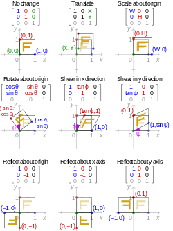
Most common geometric transformations that keep the origin fixed are linear, including rotation, scaling, shearing, reflection, and orthogonal projection; if an affine transformation is not a pure translation it keeps some point fixed, and that point can be chosen as origin to make the transformation linear. In two dimensions, linear transformations can be represented using a 2×2 transformation matrix.

Stretching

A stretch in the xy-plane is a linear transformation which enlarges all distances in a particular direction by a constant factor but does not affect distances in the perpendicular direction. We only consider stretches along the x-axis and y-axis. A stretch along the x-axis has the form x' = kx; y' = y for some positive constant k. (Note that if k> 1, then this really is a "stretch"; if k< 1, it is technically a "compression", but we still call it a stretch. Also, if k = 1, then the transformation is an identity, i.e. it has no effect.)

The matrix associated with a stretch by a factor k along the x-axis is given by:

$${\displaystyle {\begin{bmatrix}k&0\\0&1\end{bmatrix}}}$$

Similarly, a stretch by a factor k along the y-axis has the form x' = x; y' = ky, so the matrix associated with this transformation is

$${\displaystyle {\begin{bmatrix}1&0\\0&k\end{bmatrix}}}$$

Squeezing

If the two stretches above are combined with reciprocal values, then the transformation matrix represents a squeeze mapping:

$${\displaystyle {\begin{bmatrix}k&0\\0&1/k\end{bmatrix}}.}$$

A square with sides parallel to the axes is transformed to a rectangle that has the same area as the square. The reciprocal stretch and compression leave the area invariant.

Rotation

For rotation by an angle θ counterclockwise (positive direction) about the origin the functional form is ${\displaystyle x'=x\cos \theta -y\sin \theta }$ and ${\displaystyle y'=x\sin \theta +y\cos \theta }$. Written in matrix form, this becomes: ^[6]

$${\displaystyle {\begin{bmatrix}x'\\y'\end{bmatrix}}={\begin{bmatrix}\cos \theta &-\sin \theta \\\sin \theta &\cos \theta \end{bmatrix}}{\begin{bmatrix}x\\y\end{bmatrix}}}$$

Similarly, for a rotation clockwise (negative direction) about the origin, the functional form is ${\displaystyle x'=x\cos \theta +y\sin \theta }$ and ${\displaystyle y'=-x\sin \theta +y\cos \theta }$ the matrix form is:

$${\displaystyle {\begin{bmatrix}x'\\y'\end{bmatrix}}={\begin{bmatrix}\cos \theta &\sin \theta \\-\sin \theta &\cos \theta \end{bmatrix}}{\begin{bmatrix}x\\y\end{bmatrix}}}$$

These formulae assume that the x axis points right and the y axis points up.

Shearing

For shear mapping (visually similar to slanting), there are two possibilities.

A shear parallel to the x axis has ${\displaystyle x'=x+ky}$ and ${\displaystyle y'=y}$. Written in matrix form, this becomes:

$${\displaystyle {\begin{bmatrix}x'\\y'\end{bmatrix}}={\begin{bmatrix}1&k\\0&1\end{bmatrix}}{\begin{bmatrix}x\\y\end{bmatrix}}}$$

A shear parallel to the y axis has ${\displaystyle x'=x}$ and ${\displaystyle y'=y+kx}$, which has matrix form:

$${\displaystyle {\begin{bmatrix}x'\\y'\end{bmatrix}}={\begin{bmatrix}1&0\\k&1\end{bmatrix}}{\begin{bmatrix}x\\y\end{bmatrix}}}$$

Reflection

Main article: Householder transformation

For reflection about a line that goes through the origin, let ${\displaystyle \mathbf {l} =(l_{x},l_{y})}$ be a vector in the direction of the line. Then use the transformation matrix:

$${\displaystyle \mathbf {A} ={\frac {1}{\lVert \mathbf {l} \rVert ^{2}}}{\begin{bmatrix}l_{x}^{2}-l_{y}^{2}&2l_{x}l_{y}\\2l_{x}l_{y}&l_{y}^{2}-l_{x}^{2}\end{bmatrix}}}$$

Orthogonal projection

Further information: Orthogonal projection

To project a vector orthogonally onto a line that goes through the origin, let ${\displaystyle \mathbf {u} =(u_{x},u_{y})}$ be a vector in the direction of the line. Then use the transformation matrix:

$${\displaystyle \mathbf {A} ={\frac {1}{\lVert \mathbf {u} \rVert ^{2}}}{\begin{bmatrix}u_{x}^{2}&u_{x}u_{y}\\u_{x}u_{y}&u_{y}^{2}\end{bmatrix}}}$$

As with reflections, the orthogonal projection onto a line that does not pass through the origin is an affine, not linear, transformation.

Parallel projections are also linear transformations and can be represented simply by a matrix. However, perspective projections are not, and to represent these with a matrix, homogeneous coordinates can be used.

Examples in 3D computer graphics

Rotation

The matrix to rotate an angle θ about any axis defined by unit vector (x,y,z) is ^[7]

$${\displaystyle {\begin{bmatrix}xx(1-\cos \theta )+\cos \theta &yx(1-\cos \theta )-z\sin \theta &zx(1-\cos \theta )+y\sin \theta \\xy(1-\cos \theta )+z\sin \theta &yy(1-\cos \theta )+\cos \theta &zy(1-\cos \theta )-x\sin \theta \\xz(1-\cos \theta )-y\sin \theta &yz(1-\cos \theta )+x\sin \theta &zz(1-\cos \theta )+\cos \theta \end{bmatrix}}.}$$

Reflection

Main article: Householder transformation

To reflect a point through a plane ${\displaystyle ax+by+cz=0}$ (which goes through the origin), one can use ${\displaystyle \mathbf {A} =\mathbf {I} -2\mathbf {NN} ^{\mathrm {T} }}$, where ${\displaystyle \mathbf {I} }$ is the 3×3 identity matrix and ${\displaystyle \mathbf {N} }$ is the three-dimensional unit vector for the vector normal of the plane. If the L² norm of ${\displaystyle a}$, ${\displaystyle b}$, and ${\displaystyle c}$ is unity, the transformation matrix can be expressed as:

$${\displaystyle \mathbf {A} ={\begin{bmatrix}1-2a^{2}&-2ab&-2ac\\-2ab&1-2b^{2}&-2bc\\-2ac&-2bc&1-2c^{2}\end{bmatrix}}}$$

Note that these are particular cases of a Householder reflection in two and three dimensions. A reflection about a line or plane that does not go through the origin is not a linear transformation — it is an affine transformation — as a 4×4 affine transformation matrix, it can be expressed as follows (assuming the normal is a unit vector):

$${\displaystyle {\begin{bmatrix}x'\\y'\\z'\\1\end{bmatrix}}={\begin{bmatrix}1-2a^{2}&-2ab&-2ac&-2ad\\-2ab&1-2b^{2}&-2bc&-2bd\\-2ac&-2bc&1-2c^{2}&-2cd\\0&0&0&1\end{bmatrix}}{\begin{bmatrix}x\\y\\z\\1\end{bmatrix}}}$$

where ${\displaystyle d=-\mathbf {p} \cdot \mathbf {N} }$ for some point ${\displaystyle \mathbf {p} }$ on the plane, or equivalently, ${\displaystyle ax+by+cz+d=0}$.

If the 4th component of the vector is 0 instead of 1, then only the vector's direction is reflected and its magnitude remains unchanged, as if it were mirrored through a parallel plane that passes through the origin. This is a useful property as it allows the transformation of both positional vectors and normal vectors with the same matrix. See homogeneous coordinates and affine transformations below for further explanation.

Composing and inverting transformations

One of the main motivations for using matrices to represent linear transformations is that transformations can then be easily composed and inverted.

Composition is accomplished by matrix multiplication. Row and column vectors are operated upon by matrices, rows on the left and columns on the right. Since text reads from left to right, column vectors are preferred when transformation matrices are composed:

If A and B are the matrices of two linear transformations, then the effect of first applying A and then B to a column vector ${\displaystyle \mathbf {x} }$ is given by:

$${\displaystyle \mathbf {B} (\mathbf {A} \mathbf {x} )=(\mathbf {BA} )\mathbf {x} .}$$

In other words, the matrix of the combined transformation A followed by B is simply the product of the individual matrices.

When A is an invertible matrix there is a matrix A⁻¹ that represents a transformation that "undoes" A since its composition with A is the identity matrix. In some practical applications, inversion can be computed using general inversion algorithms or by performing inverse operations (that have obvious geometric interpretation, like rotating in opposite direction) and then composing them in reverse order. Reflection matrices are a special case because they are their own inverses and don't need to be separately calculated.

Other kinds of transformations

Affine transformations

Effect of applying various 2D affine transformation matrices on a unit square. Note that the reflection matrices are special cases of the scaling matrix.

Affine transformations on the 2D plane can be performed in three dimensions. Translation is done by shearing parallel to the xy plane, and rotation is performed around the z axis.

To represent affine transformations with matrices, we can use homogeneous coordinates. This means representing a 2-vector (x, y) as a 3-vector (x, y, 1), and similarly for higher dimensions. Using this system, translation can be expressed with matrix multiplication. The functional form ${\displaystyle x'=x+t_{x};y'=y+t_{y}}$ becomes:

$${\displaystyle {\begin{bmatrix}x'\\y'\\1\end{bmatrix}}={\begin{bmatrix}1&0&t_{x}\\0&1&t_{y}\\0&0&1\end{bmatrix}}{\begin{bmatrix}x\\y\\1\end{bmatrix}}.}$$

All ordinary linear transformations are included in the set of affine transformations, and can be described as a simplified form of affine transformations. Therefore, any linear transformation can also be represented by a general transformation matrix. The latter is obtained by expanding the corresponding linear transformation matrix by one row and column, filling the extra space with zeros except for the lower-right corner, which must be set to 1. For example, the counter-clockwise rotation matrix from above becomes:

$${\displaystyle {\begin{bmatrix}\cos \theta &-\sin \theta &0\\\sin \theta &\cos \theta &0\\0&0&1\end{bmatrix}}}$$

Using transformation matrices containing homogeneous coordinates, translations become linear, and thus can be seamlessly intermixed with all other types of transformations. The reason is that the real plane is mapped to the w = 1 plane in real projective space, and so translation in real Euclidean space can be represented as a shear in real projective space. Although a translation is a non-linear transformation in a 2-D or 3-D Euclidean space described by Cartesian coordinates (i.e. it can't be combined with other transformations while preserving commutativity and other properties), it becomes, in a 3-D or 4-D projective space described by homogeneous coordinates, a simple linear transformation (a shear).

More affine transformations can be obtained by composition of two or more affine transformations. For example, given a translation T' with vector ${\displaystyle (t'_{x},t'_{y}),}$ a rotation R by an angle θ counter-clockwise, a scaling S with factors ${\displaystyle (s_{x},s_{y})}$ and a translation T of vector ${\displaystyle (t_{x},t_{y}),}$ the result M of T'RST is: ^[8]

$${\displaystyle {\begin{bmatrix}s_{x}\cos \theta &-s_{y}\sin \theta &t_{x}s_{x}\cos \theta -t_{y}s_{y}\sin \theta +t'_{x}\\s_{x}\sin \theta &s_{y}\cos \theta &t_{x}s_{x}\sin \theta +t_{y}s_{y}\cos \theta +t'_{y}\\0&0&1\end{bmatrix}}}$$

When using affine transformations, the homogeneous component of a coordinate vector (normally called w) will never be altered. One can therefore safely assume that it is always 1 and ignore it. However, this is not true when using perspective projections.

Perspective projection

Main article: Perspective projection

Further information: Pinhole camera model

Comparison of the effects of applying 2D affine and perspective transformation matrices on a unit square.

Another type of transformation, of importance in 3D computer graphics, is the perspective projection. Whereas parallel projections are used to project points onto the image plane along parallel lines, the perspective projection projects points onto the image plane along lines that emanate from a single point, called the center of projection. This means that an object has a smaller projection when it is far away from the center of projection and a larger projection when it is closer (see also reciprocal function).

The simplest perspective projection uses the origin as the center of projection, and the plane at ${\displaystyle z=1}$ as the image plane. The functional form of this transformation is then ${\displaystyle x'=x/z}$; ${\displaystyle y'=y/z}$. We can express this in homogeneous coordinates as:

$${\displaystyle {\begin{bmatrix}x_{c}\\y_{c}\\z_{c}\\w_{c}\end{bmatrix}}={\begin{bmatrix}1&0&0&0\\0&1&0&0\\0&0&1&0\\0&0&1&0\end{bmatrix}}{\begin{bmatrix}x\\y\\z\\1\end{bmatrix}}={\begin{bmatrix}x\\y\\z\\z\end{bmatrix}}}$$

After carrying out the matrix multiplication, the homogeneous component ${\displaystyle w_{c}}$ will be equal to the value of ${\displaystyle z}$ and the other three will not change. Therefore, to map back into the real plane we must perform the homogeneous divide or perspective divide by dividing each component by ${\displaystyle w_{c}}$:

$${\displaystyle {\begin{bmatrix}x'\\y'\\z'\\1\end{bmatrix}}={\frac {1}{w_{c}}}{\begin{bmatrix}x_{c}\\y_{c}\\z_{c}\\w_{c}\end{bmatrix}}={\begin{bmatrix}x/z\\y/z\\1\\1\end{bmatrix}}}$$

More complicated perspective projections can be composed by combining this one with rotations, scales, translations, and shears to move the image plane and center of projection wherever they are desired.

See also

• 3D projection
• Change of basis
• Image rectification
• Pose (computer vision)
• Rigid transformation
• Transformation (function)
• Transformation geometry

References

1. Rafael Artzy (1965) Linear Geometry
2. J. W. P. Hirschfeld (1979) Projective Geometry of Finite Fields, Clarendon Press
3. Gentle, James E. (2007). "Matrix Transformations and Factorizations". Matrix Algebra: Theory, Computations, and Applications in Statistics. Springer. ISBN   9780387708737.
4. Nearing, James (2010). "Chapter 7.3 Examples of Operators" (PDF). Mathematical Tools for Physics. ISBN   978-0486482125 . Retrieved January 1, 2012.
5. Nearing, James (2010). "Chapter 7.9: Eigenvalues and Eigenvectors" (PDF). Mathematical Tools for Physics. ISBN   978-0486482125 . Retrieved January 1, 2012.
6. http://ocw.mit.edu/courses/aeronautics-and-astronautics/16-07-dynamics-fall-2009/lecture-notes/MIT16_07F09_Lec03.pdf ^{[ bare URL PDF ]}
7. Szymanski, John E. (1989). Basic Mathematics for Electronic Engineers:Models and Applications. Taylor & Francis. p. 154. ISBN   0278000681.
8. Cédric Jules (February 25, 2015). "2D transformation matrices baking".

External links

• The Matrix Page Practical examples in POV-Ray
• Reference page - Rotation of axes
• Linear Transformation Calculator
• Transformation Applet - Generate matrices from 2D transformations and vice versa.
• Coordinate transformation under rotation in 2D
• Excel Fun - Build 3D graphics from a spreadsheet