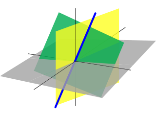
In mathematics, Gaussian elimination, also known as row reduction, is an algorithm for solving systems of linear equations. It consists of a sequence of row-wise operations performed on the corresponding matrix of coefficients. This method can also be used to compute the rank of a matrix, the determinant of a square matrix, and the inverse of an invertible matrix. The method is named after Carl Friedrich Gauss (1777–1855). To perform row reduction on a matrix, one uses a sequence of elementary row operations to modify the matrix until the lower left-hand corner of the matrix is filled with zeros, as much as possible. There are three types of elementary row operations:

Linear algebra is the branch of mathematics concerning linear equations such as:

Numerical analysis is the study of algorithms that use numerical approximation for the problems of mathematical analysis. It is the study of numerical methods that attempt to find approximate solutions of problems rather than the exact ones. Numerical analysis finds application in all fields of engineering and the physical sciences, and in the 21st century also the life and social sciences like economics, medicine, business and even the arts. Current growth in computing power has enabled the use of more complex numerical analysis, providing detailed and realistic mathematical models in science and engineering. Examples of numerical analysis include: ordinary differential equations as found in celestial mechanics, numerical linear algebra in data analysis, and stochastic differential equations and Markov chains for simulating living cells in medicine and biology.
In linear algebra, the Cholesky decomposition or Cholesky factorization is a decomposition of a Hermitian, positive-definite matrix into the product of a lower triangular matrix and its conjugate transpose, which is useful for efficient numerical solutions, e.g., Monte Carlo simulations. It was discovered by André-Louis Cholesky for real matrices, and posthumously published in 1924. When it is applicable, the Cholesky decomposition is roughly twice as efficient as the LU decomposition for solving systems of linear equations.

In numerical analysis and scientific computing, a sparse matrix or sparse array is a matrix in which most of the elements are zero. There is no strict definition regarding the proportion of zero-value elements for a matrix to qualify as sparse but a common criterion is that the number of non-zero elements is roughly equal to the number of rows or columns. By contrast, if most of the elements are non-zero, the matrix is considered dense. The number of zero-valued elements divided by the total number of elements is sometimes referred to as the sparsity of the matrix.
This is an outline of topics related to linear algebra, the branch of mathematics concerning linear equations and linear maps and their representations in vector spaces and through matrices.
In numerical analysis, the minimum degree algorithm is an algorithm used to permute the rows and columns of a symmetric sparse matrix before applying the Cholesky decomposition, to reduce the number of non-zeros in the Cholesky factor. This results in reduced storage requirements and means that the Cholesky factor can be applied with fewer arithmetic operations.
In mathematics, particularly matrix theory, a band matrix or banded matrix is a sparse matrix whose non-zero entries are confined to a diagonal band, comprising the main diagonal and zero or more diagonals on either side.
In mathematics, preconditioning is the application of a transformation, called the preconditioner, that conditions a given problem into a form that is more suitable for numerical solving methods. Preconditioning is typically related to reducing a condition number of the problem. The preconditioned problem is then usually solved by an iterative method.
In numerical analysis and linear algebra, lower–upper (LU) decomposition or factorization factors a matrix as the product of a lower triangular matrix and an upper triangular matrix. The product sometimes includes a permutation matrix as well. LU decomposition can be viewed as the matrix form of Gaussian elimination. Computers usually solve square systems of linear equations using LU decomposition, and it is also a key step when inverting a matrix or computing the determinant of a matrix. The LU decomposition was introduced by the Polish astronomer Tadeusz Banachiewicz in 1938. To quote: "It appears that Gauss and Doolittle applied the method [of elimination] only to symmetric equations. More recent authors, for example, Aitken, Banachiewicz, Dwyer, and Crout … have emphasized the use of the method, or variations of it, in connection with non-symmetric problems … Banachiewicz … saw the point … that the basic problem is really one of matrix factorization, or “decomposition” as he called it." It is also sometimes referred to as LR decomposition.
Numerical linear algebra, sometimes called applied linear algebra, is the study of how matrix operations can be used to create computer algorithms which efficiently and accurately provide approximate answers to questions in continuous mathematics. It is a subfield of numerical analysis, and a type of linear algebra. Computers use floating-point arithmetic and cannot exactly represent irrational data, so when a computer algorithm is applied to a matrix of data, it can sometimes increase the difference between a number stored in the computer and the true number that it is an approximation of. Numerical linear algebra uses properties of vectors and matrices to develop computer algorithms that minimize the error introduced by the computer, and is also concerned with ensuring that the algorithm is as efficient as possible.
In computational mathematics, a matrix-free method is an algorithm for solving a linear system of equations or an eigenvalue problem that does not store the coefficient matrix explicitly, but accesses the matrix by evaluating matrix-vector products. Such methods can be preferable when the matrix is so big that storing and manipulating it would cost a lot of memory and computing time, even with the use of methods for sparse matrices. Many iterative methods allow for a matrix-free implementation, including:
A frontal solver is an approach to solving sparse linear systems which is used extensively in finite element analysis. Algorithms of this kind are variants of Gauss elimination that automatically avoids a large number of operations involving zero terms due to the fact that the matrix is only sparse. The development of frontal solvers is usually considered as dating back to work by Bruce Irons.
In linear algebra, eigendecomposition is the factorization of a matrix into a canonical form, whereby the matrix is represented in terms of its eigenvalues and eigenvectors. Only diagonalizable matrices can be factorized in this way. When the matrix being factorized is a normal or real symmetric matrix, the decomposition is called "spectral decomposition", derived from the spectral theorem.

In mathematics, a matrix is a rectangular array or table of numbers, symbols, or expressions, with elements or entries arranged in rows and columns, which is used to represent a mathematical object or property of such an object.
In numerical analysis, nested dissection is a divide and conquer heuristic for the solution of sparse symmetric systems of linear equations based on graph partitioning. Nested dissection was introduced by George (1973); the name was suggested by Garrett Birkhoff.
In numerical mathematics, hierarchical matrices (H-matrices) are used as data-sparse approximations of non-sparse matrices. While a sparse matrix of dimension can be represented efficiently in units of storage by storing only its non-zero entries, a non-sparse matrix would require units of storage, and using this type of matrices for large problems would therefore be prohibitively expensive in terms of storage and computing time. Hierarchical matrices provide an approximation requiring only units of storage, where is a parameter controlling the accuracy of the approximation. In typical applications, e.g., when discretizing integral equations, preconditioning the resulting systems of linear equations, or solving elliptic partial differential equations, a rank proportional to with a small constant is sufficient to ensure an accuracy of . Compared to many other data-sparse representations of non-sparse matrices, hierarchical matrices offer a major advantage: the results of matrix arithmetic operations like matrix multiplication, factorization or inversion can be approximated in operations, where
Matrix Toolkit Java (MTJ) is an open-source Java software library for performing numerical linear algebra. The library contains a full set of standard linear algebra operations for dense matrices based on BLAS and LAPACK code. Partial set of sparse operations is provided through the Templates project. The library can be configured to run as a pure Java library or use BLAS machine-optimized code through the Java Native Interface.
In numerical analysis, the mixed finite element method, is a type of finite element method in which extra fields to be solved are introduced during the posing a partial differential equation problem. Somewhat related is the hybrid finite element method. The extra fields are constrained by using Lagrange multiplier fields. To be distinguished from the mixed finite element method, usual finite element methods that do not introduce such extra fields are also called irreducible or primal finite element methods. The mixed finite element method is efficient for some problems that would be numerically ill-posed if discretized by using the irreducible finite element method; one example of such problems is to compute the stress and strain fields in an almost incompressible elastic body.


