Adjacency matrix

In graph theory and computer science, an adjacency matrix is a square matrix used to represent a finite graph. The elements of the matrix indicate whether pairs of vertices are adjacent or not in the graph.

In the special case of a finite simple graph, the adjacency matrix is a (0,1)-matrix with zeros on its diagonal. If the graph is undirected (i.e. all of its edges are bidirectional), the adjacency matrix is symmetric. The relationship between a graph and the eigenvalues and eigenvectors of its adjacency matrix is studied in spectral graph theory.

The adjacency matrix of a graph should be distinguished from its incidence matrix, a different matrix representation whose elements indicate whether vertex–edge pairs are incident or not, and its degree matrix, which contains information about the degree of each vertex.

Definition

For a simple graph with vertex set U = {u₁, …, u_n}, the adjacency matrix is a square n × n matrix A such that its element A_ij is one when there is an edge from vertex u_i to vertex u_j, and zero when there is no edge. ^[1] The diagonal elements of the matrix are all zero, since edges from a vertex to itself (loops) are not allowed in simple graphs. It is also sometimes useful in algebraic graph theory to replace the nonzero elements with algebraic variables. ^[2] The same concept can be extended to multigraphs and graphs with loops by storing the number of edges between each two vertices in the corresponding matrix element, and by allowing nonzero diagonal elements. Loops may be counted either once (as a single edge) or twice (as two vertex-edge incidences), as long as a consistent convention is followed. Undirected graphs often use the latter convention of counting loops twice, whereas directed graphs typically use the former convention.

Of a bipartite graph

The adjacency matrix A of a bipartite graph whose two parts have r and s vertices can be written in the form

${\displaystyle A={\begin{pmatrix}0_{r,r}&B\\B^{\mathsf {T}}&0_{s,s}\end{pmatrix}},}$

where B is an r × s matrix, and 0_r,r and 0_s,s represent the r × r and s × s zero matrices. In this case, the smaller matrix B uniquely represents the graph, and the remaining parts of A can be discarded as redundant. B is sometimes called the biadjacency matrix.

Formally, let G = (U, V, E) be a bipartite graph with parts U = {u₁, ..., u_r}, V = {v₁, ..., v_s} and edges E. The biadjacency matrix is the r × s 0–1 matrix B in which b_i,j = 1 if and only if (u_i, v_j) ∈ E.

If G is a bipartite multigraph or weighted graph, then the elements b_i,j are taken to be the number of edges between the vertices or the weight of the edge (u_i, v_j), respectively.

Variations

An (a, b, c)-adjacency matrix A of a simple graph has A_i,j = a if (i, j) is an edge, b if it is not, and c on the diagonal. The Seidel adjacency matrix is a (−1, 1, 0)-adjacency matrix. This matrix is used in studying strongly regular graphs and two-graphs. ^[3]

The distance matrix has in position (i, j) the distance between vertices v_i and v_j. The distance is the length of a shortest path connecting the vertices. Unless lengths of edges are explicitly provided, the length of a path is the number of edges in it. The distance matrix resembles a high power of the adjacency matrix, but instead of telling only whether or not two vertices are connected (i.e., the connection matrix, which contains boolean values), it gives the exact distance between them.

Examples

Undirected graphs

The convention followed here (for undirected graphs) is that each edge adds 1 to the appropriate cell in the matrix, and each loop adds 2. ^[4] This allows the degree of a vertex to be easily found by taking the sum of the values in either its respective row or column in the adjacency matrix.

Labeled graph	Adjacency matrix
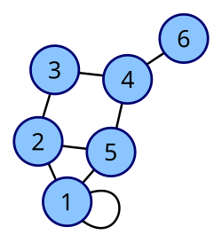	${\displaystyle {\begin{pmatrix}2&1&0&0&1&0\\1&0&1&0&1&0\\0&1&0&1&0&0\\0&0&1&0&1&1\\1&1&0&1&0&0\\0&0&0&1&0&0\end{pmatrix}}}$ Coordinates are 1–6.
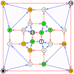
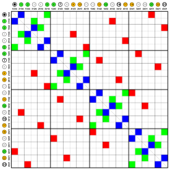
Nauru graph	Coordinates are 0–23. White fields are zeros, colored fields are ones.

Directed graphs

The adjacency matrix of a directed graph can be asymmetric. One can define the adjacency matrix of a directed graph either such that

1. a non-zero element A_ij indicates an edge from i to j or
2. it indicates an edge from j to i.

The former definition is commonly used in graph theory and social network analysis (e.g., sociology, political science, economics, psychology). ^[5] The latter is more common in other applied sciences (e.g., dynamical systems, physics, network science) where A is sometimes used to describe linear dynamics on graphs. ^[6]

Using the first definition, the in-degrees of a vertex can be computed by summing the entries of the corresponding column and the out-degree of vertex by summing the entries of the corresponding row. When using the second definition, the in-degree of a vertex is given by the corresponding row sum and the out-degree is given by the corresponding column sum.

Labeled graph	Adjacency matrix
Directed Cayley graph of S 4	Coordinates are 0–23. As the graph is directed, the matrix is not necessarily symmetric.

Trivial graphs

The adjacency matrix of a complete graph contains all ones except along the diagonal where there are only zeros. The adjacency matrix of an empty graph is a zero matrix.

Properties

Spectrum

The adjacency matrix of an undirected simple graph is symmetric, and therefore has a complete set of real eigenvalues and an orthogonal eigenvector basis. The set of eigenvalues of a graph is the spectrum of the graph. ^[7] It is common to denote the eigenvalues by ${\displaystyle \lambda _{1}\geq \lambda _{2}\geq \cdots \geq \lambda _{n}.}$

The greatest eigenvalue ${\displaystyle \lambda _{1}}$ is bounded above by the maximum degree. This can be seen as result of the Perron–Frobenius theorem, but it can be proved easily. Let v be one eigenvector associated to ${\displaystyle \lambda _{1}}$ and x the component in which v has maximum absolute value. Without loss of generality assume v_x is positive since otherwise you simply take the eigenvector ${\displaystyle -v}$, also associated to ${\displaystyle \lambda _{1}}$. Then

${\displaystyle \lambda _{1}v_{x}=(Av)_{x}=\sum _{y=1}^{n}A_{x,y}v_{y}\leq \sum _{y=1}^{n}A_{x,y}v_{x}=v_{x}\deg(x).}$

For d-regular graphs, d is the first eigenvalue of A for the vector v = (1, …, 1) (it is easy to check that it is an eigenvalue and it is the maximum because of the above bound). The multiplicity of this eigenvalue is the number of connected components of G, in particular ${\displaystyle \lambda _{1}>\lambda _{2}}$ for connected graphs. It can be shown that for each eigenvalue ${\displaystyle \lambda _{i}}$, its opposite ${\displaystyle -\lambda _{i}=\lambda _{n+1-i}}$ is also an eigenvalue of A if G is a bipartite graph. ^[8] In particular −d is an eigenvalue of any d-regular bipartite graph.

The difference ${\displaystyle \lambda _{1}-\lambda _{2}}$ is called the spectral gap and it is related to the expansion of G. It is also useful to introduce the spectral radius of ${\displaystyle A}$ denoted by ${\displaystyle \lambda (G)=\max _{\left|\lambda _{i}\right|<d}|\lambda _{i}|}$. This number is bounded by ${\displaystyle \lambda (G)\geq 2{\sqrt {d-1}}-o(1)}$. This bound is tight in the Ramanujan graphs, which have applications in many areas.

Isomorphism and invariants

Suppose two directed or undirected graphs G₁ and G₂ with adjacency matrices A₁ and A₂ are given. G₁ and G₂ are isomorphic if and only if there exists a permutation matrix P such that

${\displaystyle PA_{1}P^{-1}=A_{2}.}$

In particular, A₁ and A₂ are similar and therefore have the same minimal polynomial, characteristic polynomial, eigenvalues, determinant and trace. These can therefore serve as isomorphism invariants of graphs. However, two graphs may possess the same set of eigenvalues but not be isomorphic. ^[9] Such linear operators are said to be isospectral.

Matrix powers

If A is the adjacency matrix of the directed or undirected graph G, then the matrix Aⁿ (i.e., the matrix product of n copies of A) has an interesting interpretation: the element (i, j) gives the number of (directed or undirected) walks of length n from vertex i to vertex j. If n is the smallest nonnegative integer, such that for some i, j, the element (i, j) of Aⁿ is positive, then n is the distance between vertex i and vertex j. A great example of how this is useful is in counting the number of triangles in an undirected graph G, which is exactly the trace of A³ divided by 3 or 6 depending on whether the graph is directed or not. We divide by those values to compensate for the overcounting of each triangle. In an undirected graph, each triangle will be counted twice for all three nodes, because the path can be followed clockwise or counterclockwise : ijk or ikj. The adjacency matrix can be used to determine whether or not the graph is connected.

If a directed graph is has a nilpotent adjacency matrix (i.e., if there exists n such that Aⁿ is the zero matrix), then it is a directed acyclic graph. ^[10]

Data structures

The adjacency matrix may be used as a data structure for the representation of graphs in computer programs for manipulating graphs. The main alternative data structure, also in use for this application, is the adjacency list. ^{[11] [12]}

The space needed to represent an adjacency matrix and the time needed to perform operations on them is dependent on the matrix representation chosen for the underlying matrix. Sparse matrix representations only store non-zero matrix entries and implicitly represent the zero entries. They can, for example, be used to represent sparse graphs without incurring the space overhead from storing the many zero entries in the adjacency matrix of the sparse graph. In the following section the adjacency matrix is assumed to be represented by an array data structure so that zero and non-zero entries are all directly represented in storage.

Because each entry in the adjacency matrix requires only one bit, it can be represented in a very compact way, occupying only |V |² / 8 bytes to represent a directed graph, or (by using a packed triangular format and only storing the lower triangular part of the matrix) approximately |V |² / 16 bytes to represent an undirected graph. Although slightly more succinct representations are possible, this method gets close to the information-theoretic lower bound for the minimum number of bits needed to represent all n-vertex graphs. ^[13] For storing graphs in text files, fewer bits per byte can be used to ensure that all bytes are text characters, for instance by using a Base64 representation. ^[14] Besides avoiding wasted space, this compactness encourages locality of reference. However, for a large sparse graph, adjacency lists require less storage space, because they do not waste any space representing edges that are not present. ^{[12] [15]}

An alternative form of adjacency matrix (which, however, requires a larger amount of space) replaces the numbers in each element of the matrix with pointers to edge objects (when edges are present) or null pointers (when there is no edge). ^[15] It is also possible to store edge weights directly in the elements of an adjacency matrix. ^[12]

Besides the space tradeoff, the different data structures also facilitate different operations. Finding all vertices adjacent to a given vertex in an adjacency list is as simple as reading the list, and takes time proportional to the number of neighbors. With an adjacency matrix, an entire row must instead be scanned, which takes a larger amount of time, proportional to the number of vertices in the whole graph. On the other hand, testing whether there is an edge between two given vertices can be determined at once with an adjacency matrix, while requiring time proportional to the minimum degree of the two vertices with the adjacency list. ^{[12] [15]}

See also

• Laplacian matrix
• Self-similarity matrix

References

1. Biggs, Norman (1993), Algebraic Graph Theory, Cambridge Mathematical Library (2nd ed.), Cambridge University Press, Definition 2.1, p. 7.
2. Harary, Frank (1962), "The determinant of the adjacency matrix of a graph", SIAM Review, 4 (3): 202–210, Bibcode:1962SIAMR...4..202H, doi:10.1137/1004057, MR   0144330 .
3. Seidel, J. J. (1968). "Strongly Regular Graphs with (−1, 1, 0) Adjacency Matrix Having Eigenvalue 3". Lin. Alg. Appl. 1 (2): 281–298. doi:10.1016/0024-3795(68)90008-6.
4. Shum, Kenneth; Blake, Ian (2003-12-18). "Expander graphs and codes". Volume 68 of DIMACS series in discrete mathematics and theoretical computer science. Algebraic Coding Theory and Information Theory: DIMACS Workshop, Algebraic Coding Theory and Information Theory. American Mathematical Society. p. 63. ISBN   9780821871102.
5. Borgatti, Steve; Everett, Martin; Johnson, Jeffrey (2018), Analyzing Social Networks (2nd ed.), SAGE, p. 20
6. Newman, Mark (2018), Networks (2nd ed.), Oxford University Press, p. 110
7. Biggs (1993), Chapter 2 ("The spectrum of a graph"), pp. 7–13.
8. Brouwer, Andries E.; Haemers, Willem H. (2012), "1.3.6 Bipartite graphs", Spectra of Graphs, Universitext, New York: Springer, pp. 6–7, doi:10.1007/978-1-4614-1939-6, ISBN   978-1-4614-1938-9, MR   2882891
9. Godsil, Chris; Royle, Gordon Algebraic Graph Theory, Springer (2001), ISBN   0-387-95241-1, p.164
10. Nicholson, Victor A (1975). "Matrices with Permanent Equal to One" (PDF). Linear Algebra and its Applications (12): 187.
11. Goodrich & Tamassia (2015), p. 361: "There are two data structures that people often use to represent graphs, the adjacency list and the adjacency matrix."
12. Cormen, Thomas H.; Leiserson, Charles E.; Rivest, Ronald L.; Stein, Clifford (2001), "Section 22.1: Representations of graphs", Introduction to Algorithms (Second ed.), MIT Press and McGraw-Hill, pp. 527–531, ISBN   0-262-03293-7 .
13. Turán, György (1984), "On the succinct representation of graphs", Discrete Applied Mathematics , 8 (3): 289–294, doi:10.1016/0166-218X(84)90126-4, MR   0749658 .
14. McKay, Brendan, Description of graph6 and sparse6 encodings, archived from the original on 2001-04-30, retrieved 2012-02-10.
15. Goodrich, Michael T.; Tamassia, Roberto (2015), Algorithm Design and Applications, Wiley, p. 363.

External links

• Weisstein, Eric W. "Adjacency matrix". MathWorld .
• Fluffschack — an educational Java web start game demonstrating the relationship between adjacency matrices and graphs.
• Open Data Structures - Section 12.1 - AdjacencyMatrix: Representing a Graph by a Matrix, Pat Morin
• Café math : Adjacency Matrices of Graphs  : Application of the adjacency matrices to the computation generating series of walks.