Vector field

A portion of the vector field (sin y, sin x)

In vector calculus and physics, a vector field is an assignment of a vector to each point in a space, most commonly Euclidean space ${\displaystyle \mathbb {R} ^{n}}$. ^[1] A vector field on a plane can be visualized as a collection of arrows with given magnitudes and directions, each attached to a point on the plane. Vector fields are often used to model, for example, the speed and direction of a moving fluid throughout three dimensional space, such as the wind, or the strength and direction of some force, such as the magnetic or gravitational force, as it changes from one point to another point.

The elements of differential and integral calculus extend naturally to vector fields. When a vector field represents force, the line integral of a vector field represents the work done by a force moving along a path, and under this interpretation conservation of energy is exhibited as a special case of the fundamental theorem of calculus. Vector fields can usefully be thought of as representing the velocity of a moving flow in space, and this physical intuition leads to notions such as the divergence (which represents the rate of change of volume of a flow) and curl (which represents the rotation of a flow).

A vector field is a special case of a vector-valued function , whose domain's dimension has no relation to the dimension of its range; for example, the position vector of a space curve is defined only for smaller subset of the ambient space. Likewise, n coordinates, a vector field on a domain in n-dimensional Euclidean space ${\displaystyle \mathbb {R} ^{n}}$ can be represented as a vector-valued function that associates an n-tuple of real numbers to each point of the domain. This representation of a vector field depends on the coordinate system, and there is a well-defined transformation law ( covariance and contravariance of vectors ) in passing from one coordinate system to the other.

Vector fields are often discussed on open subsets of Euclidean space, but also make sense on other subsets such as surfaces, where they associate an arrow tangent to the surface at each point (a tangent vector). More generally, vector fields are defined on differentiable manifolds, which are spaces that look like Euclidean space on small scales, but may have more complicated structure on larger scales. In this setting, a vector field gives a tangent vector at each point of the manifold (that is, a section of the tangent bundle to the manifold). Vector fields are one kind of tensor field.

Definition

Vector fields on subsets of Euclidean space

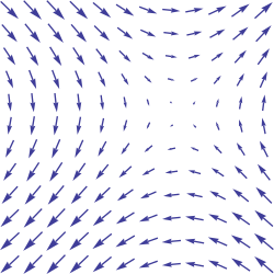
Two representations of the same vector field: v(x, y) = −r. The arrows depict the field at discrete points, however, the field exists everywhere.

Given a subset S of Rⁿ, a vector field is represented by a vector-valued function V: S → Rⁿ in standard Cartesian coordinates (x₁, …, x_n). If each component of V is continuous, then V is a continuous vector field. It is common to focus on smooth vector fields, meaning that each component is a smooth function (differentiable any number of times). A vector field can be visualized as assigning a vector to individual points within an n-dimensional space. ^[1]

One standard notation is to write ${\displaystyle {\frac {\partial }{\partial x_{1}}},\ldots ,{\frac {\partial }{\partial x_{n}}}}$ for the unit vectors in the coordinate directions. In these terms, every smooth vector field ${\displaystyle V}$ on an open subset ${\displaystyle S}$ of ${\displaystyle {\mathbf {R} }^{n}}$ can be written as

${\displaystyle \sum _{i=1}^{n}V_{i}(x_{1},\ldots ,x_{n}){\frac {\partial }{\partial x_{i}}}}$

for some smooth functions ${\displaystyle V_{1},\ldots ,V_{n}}$ on ${\displaystyle S}$. ^[2] The reason for this notation is that a vector field determines a linear map from the space of smooth functions to itself, ${\displaystyle V\colon C^{\infty }(S)\to C^{\infty }(S)}$, given by differentiating in the direction of the vector field.

Example: The vector field ${\displaystyle -x_{2}{\frac {\partial }{\partial x_{1}}}+x_{1}{\frac {\partial }{\partial x_{2}}}}$ describes a counterclockwise rotation around the origin in ${\displaystyle \mathbf {R} ^{2}}$. To show that the function ${\displaystyle x_{1}^{2}+x_{2}^{2}}$ is rotationally invariant, compute:

${\displaystyle {\bigg (}-x_{2}{\frac {\partial }{\partial x_{1}}}+x_{1}{\frac {\partial }{\partial x_{2}}}{\bigg )}(x_{1}^{2}+x_{2}^{2})=-x_{2}(2x_{1})+x_{1}(2x_{2})=0.}$

Given vector fields V, W defined on S and a smooth function f defined on S, the operations of scalar multiplication and vector addition,

$${\displaystyle (fV)(p):=f(p)V(p)}$$

$${\displaystyle (V+W)(p):=V(p)+W(p),}$$

make the smooth vector fields into a module over the ring of smooth functions, where multiplication of functions is defined pointwise.

Coordinate transformation law

In physics, a vector is additionally distinguished by how its coordinates change when one measures the same vector with respect to a different background coordinate system. The transformation properties of vectors distinguish a vector as a geometrically distinct entity from a simple list of scalars, or from a covector.

Thus, suppose that (x₁, ..., x_n) is a choice of Cartesian coordinates, in terms of which the components of the vector V are

$${\displaystyle V_{x}=(V_{1,x},\dots ,V_{n,x})}$$

and suppose that (y₁,...,y_n) are n functions of the x_i defining a different coordinate system. Then the components of the vector V in the new coordinates are required to satisfy the transformation law

$${\displaystyle V_{i,y}=\sum _{j=1}^{n}{\frac {\partial y_{i}}{\partial x_{j}}}V_{j,x}.}$$

(1)

Such a transformation law is called contravariant. A similar transformation law characterizes vector fields in physics: specifically, a vector field is a specification of n functions in each coordinate system subject to the transformation law ( 1 ) relating the different coordinate systems.

Vector fields are thus contrasted with scalar fields, which associate a number or scalar to every point in space, and are also contrasted with simple lists of scalar fields, which do not transform under coordinate changes.

Vector fields on manifolds

A vector field on a sphere

Given a differentiable manifold ${\displaystyle M}$, a vector field on ${\displaystyle M}$ is an assignment of a tangent vector to each point in ${\displaystyle M}$. ^[2] More precisely, a vector field ${\displaystyle F}$ is a mapping from ${\displaystyle M}$ into the tangent bundle ${\displaystyle TM}$ so that ${\displaystyle p\circ F}$ is the identity mapping where ${\displaystyle p}$ denotes the projection from ${\displaystyle TM}$ to ${\displaystyle M}$. In other words, a vector field is a section of the tangent bundle.

An alternative definition: A smooth vector field ${\displaystyle X}$ on a manifold ${\displaystyle M}$ is a linear map ${\displaystyle X:C^{\infty }(M)\to C^{\infty }(M)}$ such that ${\displaystyle X}$ is a derivation: ${\displaystyle X(fg)=fX(g)+X(f)g}$ for all ${\displaystyle f,g\in C^{\infty }(M)}$. ^[3]

If the manifold ${\displaystyle M}$ is smooth or analytic—that is, the change of coordinates is smooth (analytic)—then one can make sense of the notion of smooth (analytic) vector fields. The collection of all smooth vector fields on a smooth manifold ${\displaystyle M}$ is often denoted by ${\displaystyle \Gamma (TM)}$ or ${\displaystyle C^{\infty }(M,TM)}$ (especially when thinking of vector fields as sections); the collection of all smooth vector fields is also denoted by ${\textstyle {\mathfrak {X}}(M)}$ (a fraktur "X").

Examples

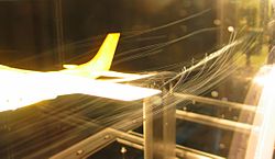
The flow field around an airplane is a vector field in R , here visualized by bubbles that follow the streamlines showing a wingtip vortex.

Vector fields are commonly used to create patterns in computer graphics. Here: abstract composition of curves following a vector field generated with OpenSimplex noise.

• A vector field for the movement of air on Earth will associate for every point on the surface of the Earth a vector with the wind speed and direction for that point. This can be drawn using arrows to represent the wind; the length (magnitude) of the arrow will be an indication of the wind speed. A "high" on the usual barometric pressure map would then act as a source (arrows pointing away), and a "low" would be a sink (arrows pointing towards), since air tends to move from high pressure areas to low pressure areas.
• Velocity field of a moving fluid. In this case, a velocity vector is associated to each point in the fluid.
• Streamlines, streaklines and pathlines are 3 types of lines that can be made from (time-dependent) vector fields. They are:
  • streaklines: the line produced by particles passing through a specific fixed point over various times
  • pathlines: showing the path that a given particle (of zero mass) would follow.
  • streamlines (or fieldlines): the path of a particle influenced by the instantaneous field (i.e., the path of a particle if the field is held fixed).
• Magnetic fields. The fieldlines can be revealed using small iron filings.
• Maxwell's equations allow us to use a given set of initial and boundary conditions to deduce, for every point in Euclidean space, a magnitude and direction for the force experienced by a charged test particle at that point; the resulting vector field is the electromagnetic field.
• A gravitational field generated by any massive object is also a vector field. For example, the gravitational field vectors for a spherically symmetric body would all point towards the sphere's center with the magnitude of the vectors reducing as radial distance from the body increases.

Gradient field in euclidean spaces

A vector field that has circulation about a point cannot be written as the gradient of a function.

Further information: Gradient

Vector fields can be constructed out of scalar fields using the gradient operator (denoted by the del: ∇). ^[4]

A vector field V defined on an open set S is called a gradient field or a conservative field if there exists a real-valued function (a scalar field) f on S such that

$${\displaystyle V=\nabla f=\left({\frac {\partial f}{\partial x_{1}}},{\frac {\partial f}{\partial x_{2}}},{\frac {\partial f}{\partial x_{3}}},\dots ,{\frac {\partial f}{\partial x_{n}}}\right).}$$

The associated flow is called the gradient flow, and is used in the method of gradient descent.

The path integral along any closed curve γ (γ(0) = γ(1)) in a conservative field is zero:

$${\displaystyle \oint _{\gamma }V(\mathbf {x} )\cdot \mathrm {d} \mathbf {x} =\oint _{\gamma }\nabla f(\mathbf {x} )\cdot \mathrm {d} \mathbf {x} =f(\gamma (1))-f(\gamma (0)).}$$

Central field in euclidean spaces

A C^∞-vector field over Rⁿ \ {0} is called a central field if

$${\displaystyle V(T(p))=T(V(p))\qquad (T\in \mathrm {O} (n,\mathbb {R} ))}$$

where O(n, R) is the orthogonal group. We say central fields are invariant under orthogonal transformations around 0.

The point 0 is called the center of the field.

Since orthogonal transformations are actually rotations and reflections, the invariance conditions mean that vectors of a central field are always directed towards, or away from, 0; this is an alternate (and simpler) definition. A central field is always a gradient field, since defining it on one semiaxis and integrating gives an antigradient.

Operations on vector fields

Line integral

Main article: Line integral

A common technique in physics is to integrate a vector field along a curve, also called determining its line integral. Intuitively this is summing up all vector components in line with the tangents to the curve, expressed as their scalar products. For example, given a particle in a force field (e.g. gravitation), where each vector at some point in space represents the force acting there on the particle, the line integral along a certain path is the work done on the particle, when it travels along this path. Intuitively, it is the sum of the scalar products of the force vector and the small tangent vector in each point along the curve.

The line integral is constructed analogously to the Riemann integral and it exists if the curve is rectifiable (has finite length) and the vector field is continuous.

Given a vector field V and a curve γ, parametrized by t in [a, b] (where a and b are real numbers), the line integral is defined as

$${\displaystyle \int _{\gamma }V(\mathbf {x} )\cdot \mathrm {d} \mathbf {x} =\int _{a}^{b}V(\gamma (t))\cdot {\dot {\gamma }}(t)\,\mathrm {d} t.}$$

To show vector field topology one can use line integral convolution.

Divergence

Main article: Divergence

The divergence of a vector field on Euclidean space is a function (or scalar field). In three-dimensions, the divergence is defined by

$${\displaystyle \operatorname {div} \mathbf {F} =\nabla \cdot \mathbf {F} ={\frac {\partial F_{1}}{\partial x}}+{\frac {\partial F_{2}}{\partial y}}+{\frac {\partial F_{3}}{\partial z}},}$$

with the obvious generalization to arbitrary dimensions. The divergence at a point represents the degree to which a small volume around the point is a source or a sink for the vector flow, a result which is made precise by the divergence theorem.

The divergence can also be defined on a Riemannian manifold, that is, a manifold with a Riemannian metric that measures the length of vectors.

Curl in three dimensions

Main article: Curl (mathematics)

The curl is an operation which takes a vector field and produces another vector field. The curl is defined only in three dimensions, but some properties of the curl can be captured in higher dimensions with the exterior derivative. In three dimensions, it is defined by

$${\displaystyle \operatorname {curl} \mathbf {F} =\nabla \times \mathbf {F} =\left({\frac {\partial F_{3}}{\partial y}}-{\frac {\partial F_{2}}{\partial z}}\right)\mathbf {e} _{1}-\left({\frac {\partial F_{3}}{\partial x}}-{\frac {\partial F_{1}}{\partial z}}\right)\mathbf {e} _{2}+\left({\frac {\partial F_{2}}{\partial x}}-{\frac {\partial F_{1}}{\partial y}}\right)\mathbf {e} _{3}.}$$

The curl measures the density of the angular momentum of the vector flow at a point, that is, the amount to which the flow circulates around a fixed axis. This intuitive description is made precise by Stokes' theorem.

Index of a vector field

The index of a vector field is an integer that helps describe its behaviour around an isolated zero (i.e., an isolated singularity of the field). In the plane, the index takes the value −1 at a saddle singularity but +1 at a source or sink singularity.

Let n be the dimension of the manifold on which the vector field is defined. Take a closed surface (homeomorphic to the (n-1)-sphere) S around the zero, so that no other zeros lie in the interior of S. A map from this sphere to a unit sphere of dimension n − 1 can be constructed by dividing each vector on this sphere by its length to form a unit length vector, which is a point on the unit sphere Sⁿ⁻¹. This defines a continuous map from S to Sⁿ⁻¹. The index of the vector field at the point is the degree of this map. It can be shown that this integer does not depend on the choice of S, and therefore depends only on the vector field itself.

The index is not defined at any non-singular point (i.e., a point where the vector is non-zero). It is equal to +1 around a source, and more generally equal to (−1)^k around a saddle that has k contracting dimensions and n−k expanding dimensions.

The index of the vector field as a whole is defined when it has just finitely many zeroes. In this case, all zeroes are isolated, and the index of the vector field is defined to be the sum of the indices at all zeroes.

For an ordinary (2-dimensional) sphere in three-dimensional space, it can be shown that the index of any vector field on the sphere must be 2. This shows that every such vector field must have a zero. This implies the hairy ball theorem.

For a vector field on a compact manifold with finitely many zeroes, the Poincaré-Hopf theorem states that the vector field’s index is the manifold’s Euler characteristic.

Physical intuition

Magnetic field lines of an iron bar (magnetic dipole)

Michael Faraday, in his concept of lines of force, emphasized that the field itself should be an object of study, which it has become throughout physics in the form of field theory.

In addition to the magnetic field, other phenomena that were modeled by Faraday include the electrical field and light field.

In recent decades many phenomenological formulations of irreversible dynamics and evolution equations in physics, from the mechanics of complex fluids and solids to chemical kinetics and quantum thermodynamics, have converged towards the geometric idea of "steepest entropy ascent" or "gradient flow" as a consistent universal modeling framework that guarantees compatibility with the second law of thermodynamics and extends well-known near-equilibrium results such as Onsager reciprocity to the far-nonequilibrium realm. ^[5]

Flow curves

Main article: Integral curve

Consider the flow of a fluid through a region of space. At any given time, any point of the fluid has a particular velocity associated with it; thus there is a vector field associated to any flow. The converse is also true: it is possible to associate a flow to a vector field having that vector field as its velocity.

Given a vector field ${\displaystyle V}$ defined on ${\displaystyle S}$, one defines curves ${\displaystyle \gamma (t)}$ on ${\displaystyle S}$ such that for each ${\displaystyle t}$ in an interval ${\displaystyle I}$,

$${\displaystyle \gamma '(t)=V(\gamma (t))\,.}$$

By the Picard–Lindelöf theorem, if ${\displaystyle V}$ is Lipschitz continuous there is a unique${\displaystyle C^{1}}$-curve ${\displaystyle \gamma _{x}}$ for each point ${\displaystyle x}$ in ${\displaystyle S}$ so that, for some ${\displaystyle \varepsilon >0}$,

$${\displaystyle {\begin{aligned}\gamma _{x}(0)&=x\\\gamma '_{x}(t)&=V(\gamma _{x}(t))\qquad \forall t\in (-\varepsilon ,+\varepsilon )\subset \mathbb {R} .\end{aligned}}}$$

The curves ${\displaystyle \gamma _{x}}$ are called integral curves or trajectories (or less commonly, flow lines) of the vector field ${\displaystyle V}$ and partition ${\displaystyle S}$ into equivalence classes. It is not always possible to extend the interval ${\displaystyle (-\varepsilon ,+\varepsilon )}$ to the whole real number line. The flow may for example reach the edge of ${\displaystyle S}$ in a finite time. In two or three dimensions one can visualize the vector field as giving rise to a flow on ${\displaystyle S}$. If we drop a particle into this flow at a point ${\displaystyle p}$ it will move along the curve ${\displaystyle \gamma _{p}}$ in the flow depending on the initial point ${\displaystyle p}$. If ${\displaystyle p}$ is a stationary point of ${\displaystyle V}$ (i.e., the vector field is equal to the zero vector at the point ${\displaystyle p}$), then the particle will remain at ${\displaystyle p}$.

Typical applications are pathline in fluid, geodesic flow, and one-parameter subgroups and the exponential map in Lie groups.

Complete vector fields

By definition, a vector field on ${\displaystyle M}$ is called complete if each of its flow curves exists for all time. ^[6] In particular, compactly supported vector fields on a manifold are complete. If ${\displaystyle X}$ is a complete vector field on ${\displaystyle M}$, then the one-parameter group of diffeomorphisms generated by the flow along ${\displaystyle X}$ exists for all time; it is described by a smooth mapping

${\displaystyle \mathbf {R} \times M\to M.}$

On a compact manifold without boundary, every smooth vector field is complete. An example of an incomplete vector field ${\displaystyle V}$ on the real line ${\displaystyle \mathbb {R} }$ is given by ${\displaystyle V(x)=x^{2}}$. For, the differential equation ${\textstyle x'(t)=x^{2}}$, with initial condition ${\displaystyle x(0)=x_{0}}$, has as its unique solution ${\textstyle x(t)={\frac {x_{0}}{1-tx_{0}}}}$ if ${\displaystyle x_{0}\neq 0}$ (and ${\displaystyle x(t)=0}$ for all ${\displaystyle t\in \mathbb {R} }$ if ${\displaystyle x_{0}=0}$). Hence for ${\displaystyle x_{0}\neq 0}$, ${\displaystyle x(t)}$ is undefined at ${\textstyle t={\frac {1}{x_{0}}}}$ so cannot be defined for all values of ${\displaystyle t}$.

The Lie bracket

The flows associated to two vector fields need not commute with each other. Their failure to commute is described by the Lie bracket of two vector fields, which is again a vector field. The Lie bracket has a simple definition in terms of the action of vector fields on smooth functions ${\displaystyle f}$:

${\displaystyle [X,Y](f):=X(Y(f))-Y(X(f)).}$

f-relatedness

Given a smooth function between manifolds, ${\displaystyle f:M\to N}$, the derivative is an induced map on tangent bundles, ${\displaystyle f_{*}:TM\to TN}$. Given vector fields ${\displaystyle V:M\to TM}$ and ${\displaystyle W:N\to TN}$, we say that ${\displaystyle W}$ is ${\displaystyle f}$-related to ${\displaystyle V}$ if the equation ${\displaystyle W\circ f=f_{*}\circ V}$ holds.

If ${\displaystyle V_{i}}$ is ${\displaystyle f}$-related to ${\displaystyle W_{i}}$, ${\displaystyle i=1,2}$, then the Lie bracket ${\displaystyle [V_{1},V_{2}]}$ is ${\displaystyle f}$-related to ${\displaystyle [W_{1},W_{2}]}$.

Generalizations

Replacing vectors by p-vectors (pth exterior power of vectors) yields p-vector fields; taking the dual space and exterior powers yields differential k-forms, and combining these yields general tensor fields.

Algebraically, vector fields can be characterized as derivations of the algebra of smooth functions on the manifold, which leads to defining a vector field on a commutative algebra as a derivation on the algebra, which is developed in the theory of differential calculus over commutative algebras.

See also

• Mathematics portal

• Eisenbud–Levine–Khimshiashvili signature formula
• Field line
• Field strength
• Gradient flow and balanced flow in atmospheric dynamics
• Lie derivative
• Scalar field
• Time-dependent vector field
• Vector fields in cylindrical and spherical coordinates
• Tensor fields

References

1. Galbis, Antonio; Maestre, Manuel (2012). Vector Analysis Versus Vector Calculus. Springer. p. 12. ISBN   978-1-4614-2199-3.
2. Tu, Loring W. (2010). "Vector fields". An Introduction to Manifolds. Springer. p. 149. ISBN   978-1-4419-7399-3.
3. Lerman, Eugene (August 19, 2011). "An Introduction to Differential Geometry" (PDF). Definition 3.23.
4. Dawber, P.G. (1987). Vectors and Vector Operators. CRC Press. p. 29. ISBN   978-0-85274-585-4.
5. Beretta, Gian Paolo (2020-05-01). "The fourth law of thermodynamics: steepest entropy ascent". Philosophical Transactions of the Royal Society A. 378 (2170): 20190168. arXiv: 1908.05768 . Bibcode:2020RSPTA.37890168B. doi:10.1098/rsta.2019.0168. ISSN   1471-2962. S2CID   201058607.
6. Sharpe, R. (1997). Differential geometry. Springer-Verlag. ISBN   0-387-94732-9.

Bibliography

• Hubbard, J. H.; Hubbard, B. B. (1999). Vector calculus, linear algebra, and differential forms. A unified approach. Upper Saddle River, NJ: Prentice Hall. ISBN   0-13-657446-7.
• Warner, Frank (1983) [1971]. Foundations of differentiable manifolds and Lie groups. New York-Berlin: Springer-Verlag. ISBN   0-387-90894-3.
• Boothby, William (1986). An introduction to differentiable manifolds and Riemannian geometry . Pure and Applied Mathematics, volume 120 (second ed.). Orlando, FL: Academic Press. ISBN   0-12-116053-X.

External links

• Online Vector Field Editor
• "Vector field", Encyclopedia of Mathematics , EMS Press, 2001 [1994]
• Vector field — Mathworld
• Vector field — PlanetMath
• 3D Magnetic field viewer
• Vector fields and field lines
• Vector field simulation An interactive application to show the effects of vector fields