Magnetic dipole

The magnetic field due to natural magnetic dipoles (upper left), magnetic monopoles (upper right), an electric current in a circular loop (lower left) or in a solenoid (lower right). All generate the same field profile when the arrangement is infinitesimally small.

In electromagnetism, a magnetic dipole is the limit of either a closed loop of electric current or a pair of poles as the size of the source is reduced to zero while keeping the magnetic moment constant.

It is a magnetic analogue of the electric dipole, but the analogy is not perfect. In particular, a true magnetic monopole, the magnetic analogue of an electric charge, has never been observed in nature. However, magnetic monopole quasiparticles have been observed as emergent properties of certain condensed matter systems. ^[2] Moreover, one form of magnetic dipole moment is associated with a fundamental quantum property—the spin of elementary particles.

Because magnetic monopoles do not exist, the magnetic field at a large distance from any static magnetic source looks like the field of a dipole with the same dipole moment. For higher-order sources (e.g. quadrupoles) with no dipole moment, their field decays towards zero with distance faster than a dipole field does.

External magnetic field produced by a magnetic dipole moment

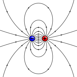
An electrostatic analogue for a magnetic moment: two opposing charges separated by a finite distance. Each arrow represents the direction of the field vector at that point.

The magnetic field of a current loop. The ring represents the current loop, which goes into the page at the x and comes out at the dot.

In classical physics, the magnetic field of a dipole is calculated as the limit of either a current loop or a pair of charges as the source shrinks to a point while keeping the magnetic moment mconstant. For the current loop, this limit is most easily derived from the vector potential: ^[3]

${\displaystyle {\mathbf {A} }({\mathbf {r} })={\frac {\mu _{0}}{4\pi r^{2}}}{\frac {{\mathbf {m} }\times {\mathbf {r} }}{r}}={\frac {\mu _{0}}{4\pi }}{\frac {{\mathbf {m} }\times {\mathbf {r} }}{r^{3}}},}$

where μ₀ is the vacuum permeability constant and 4π r² is the surface of a sphere of radius r. The magnetic flux density (strength of the B-field) is then ^[3]

${\displaystyle \mathbf {B} ({\mathbf {r} })=\nabla \times {\mathbf {A} }={\frac {\mu _{0}}{4\pi }}\left[{\frac {3\mathbf {r} (\mathbf {m} \cdot \mathbf {r} )}{r^{5}}}-{\frac {\mathbf {m} }{r^{3}}}\right].}$

Alternatively one can obtain the scalar potential first from the magnetic pole limit,

${\displaystyle \psi ({\mathbf {r} })={\frac {{\mathbf {m} }\cdot {\mathbf {r} }}{4\pi r^{3}}},}$

and hence the magnetic field strength (or strength of the H-field) is

${\displaystyle {\mathbf {H} }({\mathbf {r} })=-\nabla \psi ={\frac {1}{4\pi }}\left[{\frac {3\mathbf {\hat {r}} (\mathbf {m} \cdot \mathbf {\hat {r}} )-\mathbf {m} }{r^{3}}}\right]={\frac {\mathbf {B} }{\mu _{0}}}.}$

The magnetic field strength is symmetric under rotations about the axis of the magnetic moment. In spherical coordinates, with ${\displaystyle \mathbf {\hat {z}} =\mathbf {\hat {r}} \cos \theta -{\boldsymbol {\hat {\theta }}}\sin \theta }$, and with the magnetic moment aligned with the z-axis, then the field strength can more simply be expressed as

${\displaystyle \mathbf {H} ({\mathbf {r} })={\frac {|\mathbf {m} |}{4\pi r^{3}}}\left(2\cos \theta \,\mathbf {\hat {r}} +\sin \theta \,{\boldsymbol {\hat {\theta }}}\right).}$

Internal magnetic field of a dipole

See also: Magnetic moment § Magnetic pole definition

The two models for a dipole (current loop and magnetic poles), give the same predictions for the magnetic field far from the source. However, inside the source region they give different predictions. The magnetic field between poles is in the opposite direction to the magnetic moment (which points from the negative charge to the positive charge), while inside a current loop it is in the same direction (see the figure to the right (above for mobile users)). Clearly, the limits of these fields must also be different as the sources shrink to zero size. This distinction only matters if the dipole limit is used to calculate fields inside a magnetic material.

If a magnetic dipole is formed by making a current loop smaller and smaller, but keeping the product of current and area constant, the limiting field is

${\displaystyle \mathbf {B} (\mathbf {r} )={\frac {\mu _{0}}{4\pi }}\left[{\frac {3\mathbf {\hat {r}} (\mathbf {\hat {r}} \cdot \mathbf {m} )-\mathbf {m} }{|\mathbf {r} |^{3}}}+{\frac {8\pi }{3}}\mathbf {m} \delta (\mathbf {r} )\right],}$

where δ(r) is the Dirac delta function in three dimensions. Unlike the expressions in the previous section, this limit is correct for the internal field of the dipole.

If a magnetic dipole is formed by taking a "north pole" and a "south pole", bringing them closer and closer together but keeping the product of magnetic pole-charge and distance constant, the limiting field is

${\displaystyle \mathbf {H} (\mathbf {r} )={\frac {1}{4\pi }}\left[{\frac {3\mathbf {\hat {r}} (\mathbf {\hat {r}} \cdot \mathbf {m} )-\mathbf {m} }{|\mathbf {r} |^{3}}}-{\frac {4\pi }{3}}\mathbf {m} \delta (\mathbf {r} )\right].}$

These fields are related by B = μ₀(H + M), where

${\displaystyle \mathbf {M} (\mathbf {r} )=\mathbf {m} \delta (\mathbf {r} )}$

is the magnetization.

Forces between two magnetic dipoles

See also: Force between magnets § Magnetic dipole-dipole interaction

The force F exerted by one dipole moment m₁ on another m₂ separated in space by a vector r can be calculated using: ^[4]

${\displaystyle \mathbf {F} =\nabla \left(\mathbf {m} _{2}\cdot \mathbf {B} _{1}\right),}$

or ^{[5] [6]}

${\displaystyle \mathbf {F} (\mathbf {r} ,\mathbf {m} _{1},\mathbf {m} _{2})={\dfrac {3\mu _{0}}{4\pi r^{5}}}\left[(\mathbf {m} _{1}\cdot \mathbf {r} )\mathbf {m} _{2}+(\mathbf {m} _{2}\cdot \mathbf {r} )\mathbf {m} _{1}+(\mathbf {m} _{1}\cdot \mathbf {m} _{2})\mathbf {r} -{\dfrac {5(\mathbf {m} _{1}\cdot \mathbf {r} )(\mathbf {m} _{2}\cdot \mathbf {r} )}{r^{2}}}\mathbf {r} \right],}$

where r is the distance between dipoles. The force acting on m₁ is in the opposite direction.

The torque can be obtained from the formula

${\displaystyle {\boldsymbol {\tau }}=\mathbf {m} _{2}\times \mathbf {B} _{1}.}$

Dipolar fields from finite sources

See also: Near and far field

The magnetic scalar potential ψ produced by a finite source, but external to it, can be represented by a multipole expansion. Each term in the expansion is associated with a characteristic moment and a potential having a characteristic rate of decrease with distance r from the source. Monopole moments have a 1/r rate of decrease, dipole moments have a 1/r² rate, quadrupole moments have a 1/r³ rate, and so on. The higher the order, the faster the potential drops off. Since the lowest-order term observed in magnetic sources is the dipole term, it dominates at large distances. Therefore, at large distances any magnetic source looks like a dipole of the same magnetic moment.

Notes

1. I.S. Grant, W.R. Phillips (2008). Electromagnetism (2nd ed.). Manchester Physics, John Wiley & Sons. ISBN   978-0-471-92712-9.
2. Magnetic monopoles spotted in spin ices, September 3, 2009.
3. Chow 2006 , pp. 146–150
4. D.J. Griffiths (2007). Introduction to Electrodynamics (3rd ed.). Pearson Education. p. 276. ISBN   978-81-7758-293-2.
5. Furlani 2001 , p. 140
6. K.W. Yung; P.B. Landecker; D.D. Villani (1998). "An Analytic Solution for the Force between Two Magnetic Dipoles" (PDF). Retrieved November 24, 2012.{{cite journal}}: Cite journal requires |journal= (help)

References

• Chow, Tai L. (2006). Introduction to electromagnetic theory: a modern perspective. Jones & Bartlett Learning. ISBN   978-0-7637-3827-3.
• Jackson, John D. (1975). Classical Electrodynamics (2nd ed.). Wiley. ISBN   0-471-43132-X.
• Furlani, Edward P. (2001). Permanent Magnet and Electromechanical Devices: Materials, Analysis, and Applications. Academic Press. ISBN   0-12-269951-3.
• Schill, R. A. (2003). "General relation for the vector magnetic field of a circular current loop: A closer look". IEEE Transactions on Magnetics . 39 (2): 961–967. Bibcode:2003ITM....39..961S. doi:10.1109/TMAG.2003.808597.