Magnetic moment

Magnetic moment m of a current I, enclosing an area a.

In electromagnetism, the magnetic moment or magnetic dipole moment is the combination of strength and orientation of a magnet or other object or system that exerts a magnetic field. The magnetic dipole moment of an object determines the magnitude of torque the object experiences in a given magnetic field. When the same magnetic field is applied, objects with larger magnetic moments experience larger torques. The strength (and direction) of this torque depends not only on the magnitude of the magnetic moment but also on its orientation relative to the direction of the magnetic field. Its direction points from the south pole to north pole of the magnet (i.e., inside the magnet).

The magnetic moment also expresses the magnetic force effect of a magnet. The magnetic field of a magnetic dipole is proportional to its magnetic dipole moment. The dipole component of an object's magnetic field is symmetric about the direction of its magnetic dipole moment, and decreases as the inverse cube of the distance from the object.

Examples of objects or systems that produce magnetic moments include: permanent magnets; astronomical objects such as many planets, including the Earth, and some moons, stars, etc.; various molecules; elementary particles (e.g. electrons); composites of elementary particles (protons and neutrons —as of the nucleus of an atom); and loops of electric current such as exerted by electromagnets.

Definition, units, and measurement

Definition

The magnetic moment can be defined as a vector (really pseudovector) relating the aligning torque on the object from an externally applied magnetic field to the field vector itself. The relationship is given by: ^[1]

$${\displaystyle {\boldsymbol {\tau }}=\mathbf {m} \times \mathbf {B} }$$

where τ is the torque acting on the dipole, B is the external magnetic field, and m is the magnetic moment.

This definition is based on how one could, in principle, measure the magnetic moment of an unknown sample. For a current loop, this definition leads to the magnitude of the magnetic dipole moment equaling the product of the current times the area of the loop. Further, this definition allows the calculation of the expected magnetic moment for any known macroscopic current distribution.

An alternative definition is useful for thermodynamics calculations of the magnetic moment. In this definition, the magnetic dipole moment of a system is the negative gradient of its intrinsic energy, U_int, with respect to external magnetic field:

$${\displaystyle \mathbf {m} =-{\hat {\mathbf {x} }}{\frac {\partial U_{\text{int}}}{\partial B_{x}}}-{\hat {\mathbf {y} }}{\frac {\partial U_{\text{int}}}{\partial B_{y}}}-{\hat {\mathbf {z} }}{\frac {\partial U_{\text{int}}}{\partial B_{z}}}.}$$

Generically, the intrinsic energy includes the self-field energy of the system plus the energy of the internal workings of the system. For example, for a hydrogen atom in a 2p state in an external field, the self-field energy is negligible, so the internal energy is essentially the eigenenergy of the 2p state, which includes Coulomb potential energy and the kinetic energy of the electron. The interaction-field energy between the internal dipoles and external fields is not part of this internal energy. ^[2]

Units

The unit for magnetic moment in International System of Units (SI) base units is A⋅m², where A is ampere (SI base unit of current) and m is meter (SI base unit of distance). This unit has equivalents in other SI derived units including: ^{[3] [4]}

$${\displaystyle \mathrm {A\cdot m^{2}} ={\frac {\mathrm {N\cdot m} }{\mathrm {T} }}={\frac {\mathrm {J} }{\mathrm {T} }},}$$

where N is newton (SI derived unit of force), T is tesla (SI derived unit of magnetic flux density), and J is joule (SI derived unit of energy). ^{[5] : 20–21} Although torque (N·m) and energy (J) are dimensionally equivalent, torques are never expressed in units of energy. ^{[5] : 23}

In the CGS system, there are several different sets of electromagnetism units, of which the main ones are ESU, Gaussian, and EMU. Among these, there are two alternative (non-equivalent) units of magnetic dipole moment:

$${\displaystyle 1{\text{ statA}}{\cdot }{\text{cm}}^{2}=3.33564095\times 10^{-14}{\text{ A}}{\cdot }{\text{m}}^{2}~~{\text{ (ESU)}}}$$

$${\displaystyle 1\;{\frac {\text{erg}}{\text{G}}}=10^{-3}{\text{ A}}{\cdot }{\text{m}}^{2}~~{\text{ (Gaussian and EMU),}}}$$

where statA is statamperes, cm is centimeters, erg is ergs, and G is gauss. The ratio of these two non-equivalent CGS units (EMU/ESU) is equal to the speed of light in free space, expressed in cm⋅s ⁻¹.

All formulae in this article are correct in SI units; they may need to be changed for use in other unit systems. For example, in SI units, a loop of current with current I and area A has magnetic moment IA (see below), but in Gaussian units the magnetic moment is IA/ c .

Other units for measuring the magnetic dipole moment include the Bohr magneton and the nuclear magneton.

Measurement

Main article: magnetometer

The magnetic moments of objects are typically measured with devices called magnetometers, though not all magnetometers measure magnetic moment: Some are configured to measure magnetic field instead. If the magnetic field surrounding an object is known well enough, though, then the magnetic moment can be calculated from that magnetic field.^{[ citation needed ]}

Relation to magnetization

Main article: Magnetization

See also: Remanence

The magnetic moment is a quantity that describes the magnetic strength of an entire object. Sometimes, though, it is useful or necessary to know how much of the net magnetic moment of the object is produced by a particular portion of that magnet. Therefore, it is useful to define the magnetization field M as:

$${\displaystyle \mathbf {M} ={\frac {\mathbf {m} _{\Delta V}}{V_{\Delta V}}},}$$

where m_ΔV and V_ΔV are the magnetic dipole moment and volume of a sufficiently small portion of the magnet ΔV. This equation is often represented using derivative notation such that

$${\displaystyle \mathbf {M} ={\frac {\mathrm {d} \mathbf {m} }{\mathrm {d} V}},}$$

where dm is the elementary magnetic moment and dV is the volume element. The net magnetic moment of the magnet m therefore is

$${\displaystyle \mathbf {m} =\iiint \mathbf {M} \,\mathrm {d} V,}$$

where the triple integral denotes integration over the volume of the magnet. For uniform magnetization (where both the magnitude and the direction of M is the same for the entire magnet (such as a straight bar magnet) the last equation simplifies to:

$${\displaystyle \mathbf {m} =\mathbf {M} V,}$$

where V is the volume of the bar magnet.

The magnetization is often not listed as a material parameter for commercially available ferromagnetic materials, though. Instead the parameter that is listed is residual flux density (or remanence), denoted B_r. The formula needed in this case to calculate m in (units of A⋅m²) is:

$${\displaystyle \mathbf {m} ={\frac {1}{\mu _{0}}}\mathbf {B} _{\text{r}}V,}$$

where:

• B_r is the residual flux density, expressed in teslas.
• V is the volume of the magnet (in m³).
• μ₀ is the permeability of vacuum (4π×10⁻⁷ H/m). ^[6]

Models

The preferred classical explanation of a magnetic moment has changed over time. Before the 1930s, textbooks explained the moment using hypothetical magnetic point charges. Since then, most have defined it in terms of Ampèrian currents. ^[7] In magnetic materials, the cause of the magnetic moment are the spin and orbital angular momentum states ^{[ broken anchor ]} of the electrons, and varies depending on whether atoms in one region are aligned with atoms in another.^{[ citation needed ]}

Magnetic pole model

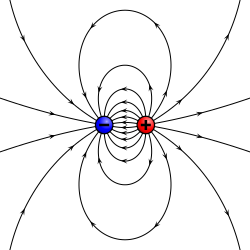
An electrostatic analog for a magnetic moment: two opposing charges separated by a finite distance.

The sources of magnetic moments in materials can be represented by poles in analogy to electrostatics. This is sometimes known as the Gilbert model. ^{[8] :  258} In this model, a small magnet is modeled by a pair of fictitious magnetic monopoles of equal magnitude but opposite polarity. Each pole is the source of magnetic force which weakens with distance. Since magnetic poles always come in pairs, their forces partially cancel each other because while one pole pulls, the other repels. This cancellation is greatest when the poles are close to each other i.e. when the bar magnet is short. The magnetic force produced by a bar magnet, at a given point in space, therefore depends on two factors: the strength p of its poles (magnetic pole strength), and the vector ${\displaystyle \mathrm {\boldsymbol {\ell }} }$ separating them. The magnetic dipole moment m is related to the fictitious poles as ^[7]

$${\displaystyle \mathbf {m} =p\,\mathrm {\boldsymbol {\ell }} \,.}$$

It points in the direction from South to North pole. The analogy with electric dipoles should not be taken too far because magnetic dipoles are associated with angular momentum (see Relation to angular momentum). Nevertheless, magnetic poles are very useful for magnetostatic calculations, particularly in applications to ferromagnets. ^[7] Practitioners using the magnetic pole approach generally represent the magnetic field by the irrotational field H, in analogy to the electric field E.

Ampèrian loop model

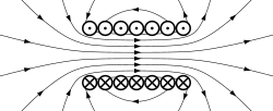
The Amperian loop model: A current loop (ring) that goes into the page at the x and comes out at the dot produces a B-field (lines). The north pole is to the right and the south to the left.

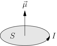
After Hans Christian Ørsted discovered that electric currents produce a magnetic field and André-Marie Ampère discovered that electric currents attract and repel each other similar to magnets, it was natural to hypothesize that all magnetic fields are due to electric current loops. In this model developed by Ampère, the elementary magnetic dipole that makes up all magnets is a sufficiently small amperian loop of current I. The dipole moment of this loop is

$${\displaystyle \mathbf {m} =I{\boldsymbol {S}},}$$

where S is the area of the loop. The direction of the magnetic moment is in a direction normal to the area enclosed by the current consistent with the direction of the current using the right hand rule.

Localized current distributions

Moment ${\displaystyle {\boldsymbol {\mu }}}$ of a planar current having magnitude I and enclosing an area S

The magnetic dipole moment can be calculated for a localized (does not extend to infinity) current distribution assuming that we know all of the currents involved. Conventionally, the derivation starts from a multipole expansion of the vector potential. This leads to the definition of the magnetic dipole moment as:

$${\displaystyle \mathbf {m} ={\tfrac {1}{2}}\iiint _{V}\mathbf {r} \times \mathbf {j} (\mathbf {r} )\,\mathrm {d} V,}$$

where × is the vector cross product, r is the position vector, and j is the electric current density and the integral is a volume integral. ^{[9] : § 5.6} When the current density in the integral is replaced by a loop of current I in a plane enclosing an area S then the volume integral becomes a line integral and the resulting dipole moment becomes

$${\displaystyle \mathbf {m} =I\mathbf {S} ,}$$

which is how the magnetic dipole moment for an Amperian loop is derived.

Practitioners using the current loop model generally represent the magnetic field by the solenoidal field B, analogous to the electrostatic field D.

Magnetic moment of a solenoid

Image of a solenoid

A generalization of the above current loop is a coil, or solenoid. Its moment is the vector sum of the moments of individual turns. If the solenoid has N identical turns (single-layer winding) and vector area S,

$${\displaystyle \mathbf {m} =NI\mathbf {S} .}$$

Quantum mechanical model

When calculating the magnetic moments of materials or molecules on the microscopic level it is often convenient to use a third model for the magnetic moment that exploits the linear relationship between the angular momentum and the magnetic moment of a particle. While this relation is straightforward to develop for macroscopic currents using the amperian loop model (see below), neither the magnetic pole model nor the amperian loop model truly represents what is occurring at the atomic and molecular levels. At that level quantum mechanics must be used. Fortunately, the linear relationship between the magnetic dipole moment of a particle and its angular momentum still holds, although it is different for each particle. Further, care must be used to distinguish between the intrinsic angular momentum (or spin) of the particle and the particle's orbital angular momentum. See below for more details.

Effects of an external magnetic field

Torque on a moment

The torque τ on an object having a magnetic dipole moment m in a uniform magnetic field B is:

$${\displaystyle {\boldsymbol {\tau }}=\mathbf {m} \times \mathbf {B} .}$$

This is valid for the moment due to any localized current distribution provided that the magnetic field is uniform. For non-uniform B the equation is also valid for the torque about the center of the magnetic dipole provided that the magnetic dipole is small enough. ^{[8] :  257}

An electron, nucleus, or atom placed in a uniform magnetic field will precess with a frequency known as the Larmor frequency. See Resonance.

Force on a moment

See also: Force between magnets

A magnetic moment in an externally produced magnetic field has a potential energy U:

$${\displaystyle U=-\mathbf {m} \cdot \mathbf {B} }$$

In a case when the external magnetic field is non-uniform, there will be a force, proportional to the magnetic field gradient, acting on the magnetic moment itself. There are two expressions for the force acting on a magnetic dipole, depending on whether the model used for the dipole is a current loop or two monopoles (analogous to the electric dipole). ^[10] The force obtained in the case of a current loop model is

$${\displaystyle \mathbf {F} _{\text{loop}}=\nabla \left(\mathbf {m} \cdot \mathbf {B} \right).}$$

Assuming existence of magnetic monopole, the force is modified as follows:

$${\displaystyle {\begin{aligned}\mathbf {F} _{\text{loop}}&=\left(\mathbf {m} \times \nabla \right)\times \mathbf {B} \\[1ex]&=\nabla \left(\mathbf {m} \cdot \mathbf {B} \right)-\left(\nabla \cdot \mathbf {B} \right)\mathbf {m} \end{aligned}}}$$

In the case of a pair of monopoles being used (i.e. electric dipole model), the force is

$${\displaystyle \mathbf {F} _{\text{dipole}}=\left(\mathbf {m} \cdot \nabla \right)\mathbf {B} .}$$

And one can be put in terms of the other via the relation

$${\displaystyle \mathbf {F} _{\text{loop}}=\mathbf {F} _{\text{dipole}}+\mathbf {m} \times \left(\nabla \times \mathbf {B} \right)-\left(\nabla \cdot \mathbf {B} \right)\mathbf {m} .}$$

In all these expressions m is the dipole and B is the magnetic field at its position. Note that if there are no currents or time-varying electrical fields or magnetic charge, ∇×B = 0, ∇⋅B = 0 and the two expressions agree.

Relation to free energy

One can relate the magnetic moment of a system to the free energy of that system. ^[11] In a uniform magnetic field B, the free energy F can be related to the magnetic moment M of the system as

$${\displaystyle \mathrm {d} F=-S\,\mathrm {d} T-\mathbf {M} \,\cdot \mathrm {d} \mathbf {B} }$$

where S is the entropy of the system and T is the temperature. Therefore, the magnetic moment can also be defined in terms of the free energy of a system as

$${\displaystyle m=\left.-{\frac {\partial F}{\partial B}}\right|_{T}.}$$

Magnetism

In addition, an applied magnetic field can change the magnetic moment of the object itself; for example by magnetizing it. This phenomenon is known as magnetism. An applied magnetic field can flip the magnetic dipoles that make up the material causing both paramagnetism and ferromagnetism. Additionally, the magnetic field can affect the currents that create the magnetic fields (such as the atomic orbits) which causes diamagnetism.

Effects on environment

Magnetic field of a magnetic moment

Main article: Magnetic dipole

See also: Dipole

Magnetic field lines around a "magnetostatic dipole". The magnetic dipole itself is located in the center of the figure, seen from the side, and pointing upward.

Any system possessing a net magnetic dipole moment m will produce a dipolar magnetic field (described below) in the space surrounding the system. While the net magnetic field produced by the system can also have higher-order multipole components, those will drop off with distance more rapidly, so that only the dipole component will dominate the magnetic field of the system at distances far away from it.

The magnetic field of a magnetic dipole depends on the strength and direction of a magnet's magnetic moment ${\displaystyle \mathbf {m} }$ but drops off as the cube of the distance such that:

$${\displaystyle \mathbf {H} (\mathbf {r} )={\frac {1}{4\pi }}\left({\frac {3\mathbf {r} (\mathbf {m} \cdot \mathbf {r} )}{|\mathbf {r} |^{5}}}-{\frac {\mathbf {m} }{|\mathbf {r} |^{3}}}\right),}$$

where ${\displaystyle \mathbf {H} }$ is the magnetic field produced by the magnet and ${\displaystyle \mathbf {r} }$ is a vector from the center of the magnetic dipole to the location where the magnetic field is measured. The inverse cube nature of this equation is more readily seen by expressing the location vector ${\displaystyle \mathbf {r} }$ as the product of its magnitude times the unit vector in its direction (${\displaystyle \mathbf {r} =|\mathbf {r} |\mathbf {\hat {r}} }$) so that:

$${\displaystyle \mathbf {H} (\mathbf {r} )={\frac {1}{4\pi }}{\frac {3\mathbf {\hat {r}} (\mathbf {\hat {r}} \cdot \mathbf {m} )-\mathbf {m} }{|\mathbf {r} |^{3}}}.}$$

The equivalent equations for the magnetic ${\displaystyle \mathbf {B} }$-field are the same except for a multiplicative factor of μ₀ = 4π×10⁻⁷  H/m , where μ₀ is known as the vacuum permeability. For example:

$${\displaystyle \mathbf {B} (\mathbf {r} )={\frac {\mu _{0}}{4\pi }}{\frac {3\mathbf {\hat {r}} (\mathbf {\hat {r}} \cdot \mathbf {m} )-\mathbf {m} }{|\mathbf {r} |^{3}}}.}$$

Forces between two magnetic dipoles

See also: Magnetic dipole–dipole interaction

As discussed earlier, the force exerted by a dipole loop with moment m₁ on another with moment m₂ is

$${\displaystyle \mathbf {F} =\nabla \left(\mathbf {m} _{2}\cdot \mathbf {B} _{1}\right),}$$

where B₁ is the magnetic field due to moment m₁. The result of calculating the gradient is ^{[12] [13]}

$${\displaystyle \mathbf {F} (\mathbf {r} ,\mathbf {m} _{1},\mathbf {m} _{2})={\frac {3\mu _{0}}{4\pi |\mathbf {r} |^{4}}}\left[\mathbf {m} _{2}(\mathbf {m} _{1}\cdot {\hat {\mathbf {r} }})+\mathbf {m} _{1}(\mathbf {m} _{2}\cdot {\hat {\mathbf {r} }})+{\hat {\mathbf {r} }}(\mathbf {m} _{1}\cdot \mathbf {m} _{2})-5{\hat {\mathbf {r} }}(\mathbf {m} _{1}\cdot {\hat {\mathbf {r} }})(\mathbf {m} _{2}\cdot {\hat {\mathbf {r} }})\right],}$$

where r̂ is the unit vector pointing from magnet 1 to magnet 2 and r is the distance. An equivalent expression is ^[13]

$${\displaystyle \mathbf {F} ={\frac {3\mu _{0}}{4\pi |\mathbf {r} |^{4}}}\left[({\hat {\mathbf {r} }}\times \mathbf {m} _{1})\times \mathbf {m} _{2}+({\hat {\mathbf {r} }}\times \mathbf {m} _{2})\times \mathbf {m} _{1}-2{\hat {\mathbf {r} }}(\mathbf {m} _{1}\cdot \mathbf {m} _{2})+5{\hat {\mathbf {r} }}({\hat {\mathbf {r} }}\times \mathbf {m} _{1})\cdot ({\hat {\mathbf {r} }}\times \mathbf {m} _{2})\right].}$$

The force acting on m₁ is in the opposite direction.

Torque of one magnetic dipole on another

The torque of magnet 1 on magnet 2 is

$${\displaystyle {\boldsymbol {\tau }}=\mathbf {m} _{2}\times \mathbf {B} _{1}.}$$

Theory underlying magnetic dipoles

Main article: Multipole expansion

See also: Magnetic dipole

The magnetic field of any magnet can be modeled by a series of terms for which each term is more complicated (having finer angular detail) than the one before it. The first three terms of that series are called the monopole (represented by an isolated magnetic north or south pole) the dipole (represented by two equal and opposite magnetic poles), and the quadrupole (represented by four poles that together form two equal and opposite dipoles). The magnitude of the magnetic field for each term decreases progressively faster with distance than the previous term, so that at large enough distances the first non-zero term will dominate.^{[ citation needed ]}

For many magnets the first non-zero term is the magnetic dipole moment. (To date, no isolated magnetic monopoles have been experimentally detected.) A magnetic dipole is the limit of either a current loop or a pair of poles as the dimensions of the source are reduced to zero while keeping the moment constant. As long as these limits only apply to fields far from the sources, they are equivalent. However, the two models give different predictions for the internal field (see below).

Magnetic potentials

Traditionally, the equations for the magnetic dipole moment (and higher order terms) are derived from theoretical quantities called magnetic potentials ^{[9] : § 5.6} which are simpler to deal with mathematically than the magnetic fields.^{[ citation needed ]}

In the magnetic pole model, the relevant magnetic field is the demagnetizing field ${\displaystyle \mathbf {H} }$. Since the demagnetizing portion of ${\displaystyle \mathbf {H} }$ does not include, by definition, the part of ${\displaystyle \mathbf {H} }$ due to free currents, there exists a magnetic scalar potential such that

$${\displaystyle {\mathbf {H} }({\mathbf {r} })=-\nabla \psi .}$$

In the amperian loop model, the relevant magnetic field is the magnetic induction ${\displaystyle \mathbf {B} }$. Since magnetic monopoles do not exist, there exists a magnetic vector potential such that

$${\displaystyle \mathbf {B} (\mathbf {r} )=\nabla \times \mathbf {A} .}$$

Both of these potentials can be calculated for any arbitrary current distribution (for the amperian loop model) or magnetic charge distribution (for the magnetic charge model) provided that these are limited to a small enough region to give:

$${\displaystyle {\begin{aligned}\mathbf {A} \left(\mathbf {r} ,t\right)&={\frac {\mu _{0}}{4\pi }}\int {\frac {\mathbf {j} \left(\mathbf {r} '\right)}{\left|\mathbf {r} -\mathbf {r} '\right|}}\,\mathrm {d} V',\\[1ex]\psi \left(\mathbf {r} ,t\right)&={\frac {1}{4\pi }}\int {\frac {\rho \left(\mathbf {r} '\right)}{\left|\mathbf {r} -\mathbf {r} '\right|}}\,\mathrm {d} V',\end{aligned}}}$$

where ${\displaystyle \mathbf {j} }$ is the current density in the amperian loop model, ${\displaystyle \rho }$ is the magnetic pole strength density in analogy to the electric charge density that leads to the electric potential, and the integrals are the volume (triple) integrals over the coordinates that make up ${\displaystyle \mathbf {r} '}$. The denominators of these equation can be expanded using the multipole expansion to give a series of terms that have larger of power of distances in the denominator. The first nonzero term, therefore, will dominate for large distances. The first non-zero term for the vector potential is:

$${\displaystyle \mathbf {A} (\mathbf {r} )={\frac {\mu _{0}}{4\pi }}{\frac {\mathbf {m} \times \mathbf {r} }{|\mathbf {r} |^{3}}},}$$

where ${\displaystyle \mathbf {m} }$ is:

$${\displaystyle \mathbf {m} ={\frac {1}{2}}\iiint _{V}\mathbf {r} \times \mathbf {j} \,\mathrm {d} V,}$$

where × is the vector cross product, r is the position vector, and j is the electric current density and the integral is a volume integral.

In the magnetic pole perspective, the first non-zero term of the scalar potential is

$${\displaystyle \psi (\mathbf {r} )={\frac {\mathbf {m} \cdot \mathbf {r} }{4\pi |\mathbf {r} |^{3}}}.}$$

Here ${\displaystyle \mathbf {m} }$ may be represented in terms of the magnetic pole strength density but is more usefully expressed in terms of the magnetization field as:

$${\displaystyle \mathbf {m} =\iiint \mathbf {M} \,\mathrm {d} V.}$$

The same symbol ${\displaystyle \mathbf {m} }$ is used for both equations since they produce equivalent results outside of the magnet.

External magnetic field produced by a magnetic dipole moment

The magnetic flux density for a magnetic dipole in the amperian loop model, therefore, is

$${\displaystyle \mathbf {B} (\mathbf {r} )=\nabla \times {\mathbf {A} }={\frac {\mu _{0}}{4\pi }}\left({\frac {3\mathbf {r} (\mathbf {m} \cdot \mathbf {r} )}{|\mathbf {r} |^{5}}}-{\frac {\mathbf {m} }{|\mathbf {r} |^{3}}}\right).}$$

Further, the magnetic field strength ${\displaystyle \mathbf {H} }$ is

$${\displaystyle {\mathbf {H} }({\mathbf {r} })=-\nabla \psi ={\frac {1}{4\pi }}\left({\frac {3\mathbf {r} (\mathbf {m} \cdot \mathbf {r} )}{|\mathbf {r} |^{5}}}-{\frac {\mathbf {m} }{|\mathbf {r} |^{3}}}\right).}$$

Internal magnetic field of a dipole

The magnetic field of a current loop

The two models for a dipole (magnetic poles or current loop) give the same predictions for the magnetic field far from the source. However, inside the source region, they give different predictions. The magnetic field between poles (see the figure for Magnetic pole model) is in the opposite direction to the magnetic moment (which points from the negative charge to the positive charge), while inside a current loop it is in the same direction (see the figure to the right). The limits of these fields must also be different as the sources shrink to zero size. This distinction only matters if the dipole limit is used to calculate fields inside a magnetic material. ^[7]

If a magnetic dipole is formed by taking a "north pole" and a "south pole", bringing them closer and closer together but keeping the product of magnetic pole charge and distance constant, the limiting field is ^[7]

$${\displaystyle \mathbf {H} (\mathbf {r} )={\frac {1}{4\pi }}\left[{\frac {3\mathbf {\hat {r}} (\mathbf {\hat {r}} \cdot \mathbf {m} )-\mathbf {m} }{|\mathbf {r} |^{3}}}-{\frac {4\pi }{3}}\mathbf {m} \delta (\mathbf {r} )\right].}$$

If a magnetic dipole is formed by making a current loop smaller and smaller, but keeping the product of current and area constant, the limiting field is

$${\displaystyle \mathbf {B} (\mathbf {r} )={\frac {\mu _{0}}{4\pi }}\left[{\frac {3\mathbf {\hat {r}} (\mathbf {\hat {r}} \cdot \mathbf {m} )-\mathbf {m} }{|\mathbf {r} |^{3}}}+{\frac {8\pi }{3}}\mathbf {m} \delta (\mathbf {r} )\right].}$$

Unlike the expressions in the previous section, this limit is correct for the internal field of the dipole. ^{[7] [9] :  184}

These fields are related by B = μ₀(H + M), where M(r) = mδ(r) is the magnetization.

Relation to angular momentum

See also: gyromagnetic ratio

The magnetic moment has a close connection with angular momentum called the gyromagnetic effect. This effect is expressed on a macroscopic scale in the Einstein–de Haas effect, or "rotation by magnetization", and its inverse, the Barnett effect, or "magnetization by rotation". ^[1] Further, a torque applied to a relatively isolated magnetic dipole such as an atomic nucleus can cause it to precess (rotate about the axis of the applied field). This phenomenon is used in nuclear magnetic resonance.^{[ citation needed ]}

Viewing a magnetic dipole as current loop brings out the close connection between magnetic moment and angular momentum. Since the particles creating the current (by rotating around the loop) have charge and mass, both the magnetic moment and the angular momentum increase with the rate of rotation. The ratio of the two is called the gyromagnetic ratio or ${\displaystyle \gamma }$ so that: ^{[14] [15]}

$${\displaystyle \mathbf {m} =\gamma \,\mathbf {L} ,}$$

where ${\displaystyle \mathbf {L} }$ is the angular momentum of the particle or particles that are creating the magnetic moment.

In the amperian loop model, which applies for macroscopic currents, the gyromagnetic ratio is one half of the charge-to-mass ratio. This can be shown as follows. The angular momentum of a moving charged particle is defined as:

$${\displaystyle \mathbf {L} =\mathbf {r} \times \mathbf {p} =\mu \,\mathbf {r} \times \mathbf {v} ,}$$

where μ is the mass of the particle and v is the particle's velocity. The angular momentum of the very large number of charged particles that make up a current therefore is:

$${\displaystyle \mathbf {L} =\iiint _{V}\,\mathbf {r} \times (\rho \mathbf {v} )\,\mathrm {d} V\,,}$$

where ρ is the mass density of the moving particles. By convention the direction of the cross product is given by the right-hand rule. ^[16]

This is similar to the magnetic moment created by the very large number of charged particles that make up that current:

$${\displaystyle \mathbf {m} ={\tfrac {1}{2}}\iiint _{V}\mathbf {r} \times (\rho _{Q}\mathbf {v} )\,\mathrm {d} V\,,}$$

where ${\displaystyle \mathbf {j} =\rho _{Q}\mathbf {v} }$ and ${\displaystyle \rho _{Q}}$ is the charge density of the moving charged particles.

Comparing the two equations results in:

$${\displaystyle \mathbf {m} ={\frac {e}{2\mu }}\,\mathbf {L} \,,}$$

where ${\displaystyle e}$ is the charge of the particle and ${\displaystyle \mu }$ is the mass of the particle.

Even though atomic particles cannot be accurately described as orbiting (and spinning) charge distributions of uniform charge-to-mass ratio, this general trend can be observed in the atomic world so that:

$${\displaystyle \mathbf {m} =g\,{\frac {e}{2\mu }}\,\mathbf {L} ,}$$

where the g-factor depends on the particle and configuration. For example, the g-factor for the magnetic moment due to an electron orbiting a nucleus is one while the g-factor for the magnetic moment of electron due to its intrinsic angular momentum (spin) is a little larger than 2. The g-factor of atoms and molecules must account for the orbital and intrinsic moments of its electrons and possibly the intrinsic moment of its nuclei as well.

In the atomic world the angular momentum (spin) of a particle is an integer (or half-integer in the case of fermions) multiple of the reduced Planck constant ħ. This is the basis for defining the magnetic moment units of Bohr magneton (assuming charge-to-mass ratio of the electron) and nuclear magneton (assuming charge-to-mass ratio of the proton). See electron magnetic moment and Bohr magneton for more details.

Atoms, molecules, and elementary particles

Fundamentally, contributions to any system's magnetic moment may come from sources of two kinds: 1) motion of electric charges, such as electric currents; and 2) the intrinsic magnetism due spin of elementary particles, such as the electron.^{[ citation needed ]}

Contributions due to the sources of the first kind can be calculated from knowing the distribution of all the electric currents (or, alternatively, of all the electric charges and their velocities) inside the system, by using the formulas below.

Contributions due to particle spin sum the magnitude of each elementary particle's intrinsic magnetic moment, a fixed number, often measured experimentally to a great precision. For example, any electron's magnetic moment is measured to be −9.284764×10⁻²⁴ J/T. ^[17] The direction of the magnetic moment of any elementary particle is entirely determined by the direction of its spin, with the negative value indicating that any electron's magnetic moment is antiparallel to its spin.

The net magnetic moment of any system is a vector sum of contributions from one or both types of sources. For example, the magnetic moment of an atom of hydrogen-1 (the lightest hydrogen isotope, consisting of a proton and an electron) is a vector sum of the following contributions:

1. the intrinsic moment of the electron,
2. the orbital motion of the electron around the proton,
3. the intrinsic moment of the proton.

Similarly, the magnetic moment of a bar magnet is the sum of the contributing magnetic moments, which include the intrinsic and orbital magnetic moments of the unpaired electrons of the magnet's material and the nuclear magnetic moments.

Magnetic moment of an atom

For an atom, individual electron spins are added to get a total spin, and individual orbital angular momenta are added to get a total orbital angular momentum. These two then are added using angular momentum coupling to get a total angular momentum. For an atom with no nuclear magnetic moment, the magnitude of the atomic dipole moment, ${\displaystyle {\mathfrak {m}}_{\text{atom}}}$, is then ^[18]

$${\displaystyle {\mathfrak {m}}_{\text{atom}}=g_{\text{J}}\,\mu _{\text{B}}\,{\sqrt {j\,(j+1)\,}}}$$

where j is the total angular momentum quantum number, g_J is the Landé g-factor, and μ_B is the Bohr magneton. The component of this magnetic moment along the direction of the magnetic field is then ^[19]

$${\displaystyle {\mathfrak {m}}_{{\text{atom}},z}=-m\,g_{\text{J}}\,\mu _{\text{B}}\,.}$$

The negative sign occurs because electrons have negative charge.

The integer m (not to be confused with the moment, ${\displaystyle {\mathfrak {m}}}$) is called the magnetic quantum number or the equatorial quantum number, which can take on any of 2j + 1 values: ^[20]

$${\displaystyle -j,\ -(j-1),\ \cdots ,\ -1,\ 0,\ +1,\ \cdots ,\ +(j-1),\ +j~.}$$

Due to the angular momentum, the dynamics of a magnetic dipole in a magnetic field differs from that of an electric dipole in an electric field. The field does exert a torque on the magnetic dipole tending to align it with the field. However, torque is proportional to rate of change of angular momentum, so precession occurs: the direction of spin changes. This behavior is described by the Landau–Lifshitz–Gilbert equation: ^{[21] [22]}

$${\displaystyle {\frac {1}{\gamma }}{\frac {\mathrm {d} \mathbf {m} }{\mathrm {d} t}}=\mathbf {m} \times \mathbf {H} _{\text{eff}}-{\frac {\lambda }{\gamma m}}\mathbf {m} \times {\frac {\mathrm {d} \mathbf {m} }{\mathrm {d} t}}}$$

where γ is the gyromagnetic ratio, m is the magnetic moment, λ is the damping coefficient and H_eff is the effective magnetic field (the external field plus any self-induced field). The first term describes precession of the moment about the effective field, while the second is a damping term related to dissipation of energy caused by interaction with the surroundings.

Magnetic moment of an electron

See also: Anomalous magnetic dipole moment and Electron magnetic moment

Electrons and many elementary particles also have intrinsic magnetic moments, an explanation of which requires a quantum mechanical treatment and relates to the intrinsic angular momentum of the particles as discussed in the article Electron magnetic moment. It is these intrinsic magnetic moments that give rise to the macroscopic effects of magnetism, and other phenomena, such as electron paramagnetic resonance.^{[ citation needed ]}

The magnetic moment of the electron is

$${\displaystyle \mathbf {m} _{\text{S}}=-{\frac {g_{\text{S}}\mu _{\text{B}}\mathbf {S} }{\hbar }},}$$

where μ_B is the Bohr magneton, S is electron spin, and the g-factor g_S is 2 according to Dirac's theory, but due to quantum electrodynamic effects it is slightly larger in reality: 2.00231930436. The deviation from 2 is known as the anomalous magnetic dipole moment.

Again it is important to notice that m is a negative constant multiplied by the spin, so the magnetic moment of the electron is antiparallel to the spin. This can be understood with the following classical picture: if we imagine that the spin angular momentum is created by the electron mass spinning around some axis, the electric current that this rotation creates circulates in the opposite direction, because of the negative charge of the electron; such current loops produce a magnetic moment which is antiparallel to the spin. Hence, for a positron (the anti-particle of the electron) the magnetic moment is parallel to its spin.

Magnetic moment of a nucleus

See also: Nucleon magnetic moment and Nuclear magnetic moment

The nuclear system is a complex physical system consisting of nucleons, i.e., protons and neutrons. The quantum mechanical properties of the nucleons include the spin among others. Since the electromagnetic moments of the nucleus depend on the spin of the individual nucleons, one can look at these properties with measurements of nuclear moments, and more specifically the nuclear magnetic dipole moment.

Most common nuclei exist in their ground state, although nuclei of some isotopes have long-lived excited states. Each energy state of a nucleus of a given isotope is characterized by a well-defined magnetic dipole moment, the magnitude of which is a fixed number, often measured experimentally to a great precision. This number is very sensitive to the individual contributions from nucleons, and a measurement or prediction of its value can reveal important information about the content of the nuclear wave function. There are several theoretical models that predict the value of the magnetic dipole moment and a number of experimental techniques aiming to carry out measurements in nuclei along the nuclear chart.

Magnetic moment of a molecule

Any molecule has a well-defined magnitude of magnetic moment, which may depend on the molecule's energy state. Typically, the overall magnetic moment of a molecule is a combination of the following contributions, in the order of their typical strength:

• magnetic moments due to its unpaired electron spins (paramagnetic contribution), if any
• orbital motion of its electrons, which in the ground state is often proportional to the external magnetic field (diamagnetic contribution)
• the combined magnetic moment of its nuclear spins, which depends on the nuclear spin configuration.

Examples of molecular magnetism

• The dioxygen molecule, O₂, exhibits strong paramagnetism, due to unpaired spins of its outermost two electrons.
• The carbon dioxide molecule, CO₂, mostly exhibits diamagnetism, a much weaker magnetic moment of the electron orbitals that is proportional to the external magnetic field. The nuclear magnetism of a magnetic isotope such as ¹³C or ¹⁷O will contribute to the molecule's magnetic moment.
• The dihydrogen molecule, H₂, in a weak (or zero) magnetic field exhibits nuclear magnetism, and can be in a para- or an ortho- nuclear spin configuration.
• Many transition metal complexes are magnetic. The spin-only formula is a good first approximation for high-spin complexes of first-row transition metals. ^[23]

Number of unpaired electrons	Spin-only moment ( μB )
1	1.73
2	2.83
3	3.87
4	4.90
5	5.92

Elementary particles

In atomic and nuclear physics, the Greek symbol μ represents the magnitude of the magnetic moment, often measured in Bohr magnetons or nuclear magnetons, associated with the intrinsic spin of the particle and/or with the orbital motion of the particle in a system. Values of the intrinsic magnetic moments of some particles are given in the table below:

Intrinsic magnetic moments and spins
of some elementary particles ^[24]

Particle name (symbol)	Magnetic dipole moment (10−27  J⋅T −1)	Spin quantum number (dimensionless)
electron (e−)	−9284.764	1/2
proton (H+)	–0 014.106067	1/2
neutron (n)	0 00−9.66236	1/2
muon (μ−)	0 0−44.904478	1/2
deuteron (2H+)	–0 004.3307346	1
triton (3H+)	–0 015.046094	1/2
helion (3He++)	0 0−10.746174	1/2
alpha particle (4He++)	–0 000	0

See also

• Moment (physics)
• Electric dipole moment
• Toroidal dipole moment
• Magnetic susceptibility
• Orbital magnetization
• Magnetic dipole–dipole interaction

References and notes

1. Cullity, B. D.; Graham, C. D. (2008). Introduction to Magnetic Materials (2nd ed.). Wiley-IEEE Press. p. 103. ISBN   978-0-471-47741-9.
2. See, for example, Callen, Herbert B. (1985). Thermodynamics and an Introduction to Thermostatistics (2nd ed.). John Wiley & Sons. p.  200. ISBN   978-0-471-86256-7. where the relevant U is U[B_e].
3. "Magnetic units". IEEE Magnetics. Retrieved 19 February 2016.
4. Mohr, Peter J.; Newell, David B.; Taylor, Barry N. (21 Jul 2015). "CODATA Recommended Values of the Fundamental Physical Constants: 2014". Reviews of Modern Physics. 88 (3): 035009. arXiv: 1507.07956 . Bibcode:2016RvMP...88c5009M. doi:10.1103/RevModPhys.88.035009. S2CID   1115862.
5. Le Système international d’unités [The International System of Units](PDF) (in French and English) (9th ed.), International Bureau of Weights and Measures, 2019, ISBN   978-92-822-2272-0
6. "K&J Magnetics – Glossary". www.kjmagnetics.com.
7. Brown, William Fuller Jr. (1962). Magnetostatic Principles in Ferromagnetism. North-Holland.
8. Griffiths, David J. (1999). Introduction to Electrodynamics (3rd ed.). Prentice Hall. p. 258. ISBN   978-0-13-805326-0. OCLC   40251748.
9. Jackson, John David (1975). Classical Electrodynamics (2 ed.). Wiley. ISBN   978-0-471-43132-9.
10. Boyer, Timothy H. (1988). "The Force on a Magnetic Dipole". Am. J. Phys. 56 (8): 688–692. Bibcode:1988AmJPh..56..688B. doi:10.1119/1.15501.
11. Landau, L. D.; Lifshitz, E. M.; Pitaevskii, L. P. (January 15, 1984). Electrodynamics of Continuous Media: Volume 8 (Course of Theoretical Physics) (2 ed.). Butterworth-Heinemann. p. 130. ISBN   978-0-7506-2634-7.
12. Furlani, Edward P. (2001). Permanent Magnet and Electromechanical Devices: Materials, Analysis, and Applications. Academic Press. p. 140. ISBN   978-0-12-269951-1.
13. Yung, K. W.; Landecker, P. B.; Villani, D. D. (1998). "An Analytic Solution for the Force between Two Magnetic Dipoles" (PDF). Magnetic and Electrical Separation. 9: 39–52. doi: 10.1155/1998/79537 . Retrieved November 24, 2012.
14. Krey, Uwe; Owen, Anthony (2007). Basic Theoretical Physics. Springer. pp. 151–152. ISBN   978-3-540-36804-5.
15. Buxton, Richard B. (2002). Introduction to functional magnetic resonance imaging. Cambridge University Press. p. 136. ISBN   978-0-521-58113-4.
16. Feynman, Richard P.; Leighton, Robert B.; Sands, Matthew (2006). The Feynman Lectures on Physics. Vol. 2. Pearson/Addison-Wesley. pp. 13–12. ISBN   978-0-8053-9045-2.
17. "CODATA Value: electron magnetic moment". physics.nist.gov.
18. Tilley, R. J. D. (2004). Understanding Solids. John Wiley and Sons. p. 368. ISBN   978-0-470-85275-0.
19. Tipler, Paul Allen; Llewellyn, Ralph A. (2002). Modern Physics (4th ed.). Macmillan. p. 310. ISBN   978-0-7167-4345-3.
20. Crowther, J.A. (1949). Ions, Electrons, and Ionizing Radiations (8th ed.). London: Edward Arnold. p.  270.
21. Rice, Stuart Alan (2004). Advances in chemical physics. Wiley. pp. 208ff. ISBN   978-0-471-44528-9.
22. Steiner, Marcus (2004). Micromagnetism and Electrical Resistance of Ferromagnetic Electrodes for Spin Injection Devices. Cuvillier Verlag. p. 6. ISBN   978-3-86537-176-8.
23. Figgis, B.N.; Lewis, J. (1960). "The magnetochemistry of complex compounds". In Lewis, J.; Wilkins, R.G. (eds.). Modern Coordination Chemistry: Principles and methods. New York: Interscience. pp. 405–407.
24. "Search results matching 'magnetic moment'". CODATA internationally recommended values of the Fundamental Physical Constants. National Institute of Standards and Technology. Retrieved 11 May 2012.

External links

• Bowtell, Richard (2009). "μ – Magnetic Moment". Sixty Symbols. Brady Haran for the University of Nottingham.