In quantum mechanics, the Hamiltonian of a system is an operator corresponding to the total energy of that system, including both kinetic energy and potential energy. Its spectrum, the system's energy spectrum or its set of energy eigenvalues, is the set of possible outcomes obtainable from a measurement of the system's total energy. Due to its close relation to the energy spectrum and time-evolution of a system, it is of fundamental importance in most formulations of quantum theory.
The mathematical formulations of quantum mechanics are those mathematical formalisms that permit a rigorous description of quantum mechanics. This mathematical formalism uses mainly a part of functional analysis, especially Hilbert spaces, which are a kind of linear space. Such are distinguished from mathematical formalisms for physics theories developed prior to the early 1900s by the use of abstract mathematical structures, such as infinite-dimensional Hilbert spaces, and operators on these spaces. In brief, values of physical observables such as energy and momentum were no longer considered as values of functions on phase space, but as eigenvalues; more precisely as spectral values of linear operators in Hilbert space.

The quantum harmonic oscillator is the quantum-mechanical analog of the classical harmonic oscillator. Because an arbitrary smooth potential can usually be approximated as a harmonic potential at the vicinity of a stable equilibrium point, it is one of the most important model systems in quantum mechanics. Furthermore, it is one of the few quantum-mechanical systems for which an exact, analytical solution is known.

The Schrödinger equation is a partial differential equation that governs the wave function of a quantum-mechanical system. Its discovery was a significant landmark in the development of quantum mechanics. It is named after Erwin Schrödinger, who postulated the equation in 1925 and published it in 1926, forming the basis for the work that resulted in his Nobel Prize in Physics in 1933.
In quantum chemistry and molecular physics, the Born–Oppenheimer (BO) approximation is the best-known mathematical approximation in molecular dynamics. Specifically, it is the assumption that the wave functions of atomic nuclei and electrons in a molecule can be treated separately, based on the fact that the nuclei are much heavier than the electrons. Due to the larger relative mass of a nucleus compared to an electron, the coordinates of the nuclei in a system are approximated as fixed, while the coordinates of the electrons are dynamic. The approach is named after Max Born and his 23-year-old graduate student J. Robert Oppenheimer, the latter of whom proposed it in 1927 during a period of intense fervent in the development of quantum mechanics.

Quantum superposition is a fundamental principle of quantum mechanics that states that linear combinations of solutions to the Schrödinger equation are also solutions of the Schrödinger equation. This follows from the fact that the Schrödinger equation is a linear differential equation in time and position. More precisely, the state of a system is given by a linear combination of all the eigenfunctions of the Schrödinger equation governing that system.

The ground state of a quantum-mechanical system is its stationary state of lowest energy; the energy of the ground state is known as the zero-point energy of the system. An excited state is any state with energy greater than the ground state. In quantum field theory, the ground state is usually called the vacuum state or the vacuum.

In quantum mechanics, the azimuthal quantum numberℓ is a quantum number for an atomic orbital that determines its orbital angular momentum and describes aspects of the angular shape of the orbital. The azimuthal quantum number is the second of a set of quantum numbers that describe the unique quantum state of an electron.

In physics, the Rabi cycle is the cyclic behaviour of a two-level quantum system in the presence of an oscillatory driving field. A great variety of physical processes belonging to the areas of quantum computing, condensed matter, atomic and molecular physics, and nuclear and particle physics can be conveniently studied in terms of two-level quantum mechanical systems, and exhibit Rabi flopping when coupled to an optical driving field. The effect is important in quantum optics, magnetic resonance and quantum computing, and is named after Isidor Isaac Rabi.
The adiabatic theorem is a concept in quantum mechanics. Its original form, due to Max Born and Vladimir Fock (1928), was stated as follows:
In quantum mechanics, a rotational transition is an abrupt change in angular momentum. Like all other properties of a quantum particle, angular momentum is quantized, meaning it can only equal certain discrete values, which correspond to different rotational energy states. When a particle loses angular momentum, it is said to have transitioned to a lower rotational energy state. Likewise, when a particle gains angular momentum, a positive rotational transition is said to have occurred.
In physics, a free particle is a particle that, in some sense, is not bound by an external force, or equivalently not in a region where its potential energy varies. In classical physics, this means the particle is present in a "field-free" space. In quantum mechanics, it means the particle is in a region of uniform potential, usually set to zero in the region of interest since the potential can be arbitrarily set to zero at any point in space.

In quantum mechanics, a two-state system is a quantum system that can exist in any quantum superposition of two independent quantum states. The Hilbert space describing such a system is two-dimensional. Therefore, a complete basis spanning the space will consist of two independent states. Any two-state system can also be seen as a qubit.

Quantum orbital motion involves the quantum mechanical motion of rigid particles about some other mass, or about themselves. In classical mechanics, an object's orbital motion is characterized by its orbital angular momentum and spin angular momentum, which is the object's angular momentum about its own center of mass. In quantum mechanics there are analogous orbital and spin angular momenta which describe the orbital motion of a particle, represented as quantum mechanical operators instead of vectors.
In quantum mechanics, the Hellmann–Feynman theorem relates the derivative of the total energy with respect to a parameter to the expectation value of the derivative of the Hamiltonian with respect to that same parameter. According to the theorem, once the spatial distribution of the electrons has been determined by solving the Schrödinger equation, all the forces in the system can be calculated using classical electrostatics.
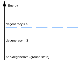
In quantum mechanics, an energy level is degenerate if it corresponds to two or more different measurable states of a quantum system. Conversely, two or more different states of a quantum mechanical system are said to be degenerate if they give the same value of energy upon measurement. The number of different states corresponding to a particular energy level is known as the degree of degeneracy of the level. It is represented mathematically by the Hamiltonian for the system having more than one linearly independent eigenstate with the same energy eigenvalue. When this is the case, energy alone is not enough to characterize what state the system is in, and other quantum numbers are needed to characterize the exact state when distinction is desired. In classical mechanics, this can be understood in terms of different possible trajectories corresponding to the same energy.
A normalized 1s Slater-type function is a function which is used in the descriptions of atoms and in a broader way in the description of atoms in molecules. It is particularly important as the accurate quantum theory description of the smallest free atom, hydrogen. It has the form
In quantum mechanics, the eigenvalue of an observable is said to be a good quantum number if the observable is a constant of motion. In other words, the quantum number is good if the corresponding observable commutes with the Hamiltonian. If the system starts from the eigenstate with an eigenvalue , it remains on that state as the system evolves in time, and the measurement of always yields the same eigenvalue .
In quantum mechanics, energy is defined in terms of the energy operator, acting on the wave function of the system as a consequence of time translation symmetry.
This is a glossary for the terminology often encountered in undergraduate quantum mechanics courses.


![Three wavefunction solutions to the time-dependent Schrodinger equation for a harmonic oscillator. Left: The real part (blue) and imaginary part (red) of the wavefunction. Right: The probability of finding the particle at a certain position. The top two rows are two stationary states, and the bottom is the superposition state
ps
N
[?]
(
ps
0
+
ps
1
)
/
2
{\textstyle \psi _{N}\equiv (\psi _{0}+\psi _{1})/{\sqrt {2}}}
, which is not a stationary state. The right column illustrates why stationary states are called "stationary". StationaryStatesAnimation.gif](http://upload.wikimedia.org/wikipedia/commons/e/e0/StationaryStatesAnimation.gif)


