Maxwell stress tensor

The Maxwell stress tensor (named after James Clerk Maxwell) is a symmetric second-order tensor in three dimensions that is used in classical electromagnetism to represent the interaction between electromagnetic forces and mechanical momentum. In simple situations, such as a point charge moving freely in a homogeneous magnetic field, it is easy to calculate the forces on the charge from the Lorentz force law. When the situation becomes more complicated, this ordinary procedure can become impractically difficult, with equations spanning multiple lines. It is therefore convenient to collect many of these terms in the Maxwell stress tensor, and to use tensor arithmetic to find the answer to the problem at hand.

In the relativistic formulation of electromagnetism, the nine components of the Maxwell stress tensor appear, negated, as components of the electromagnetic stress–energy tensor, which is the electromagnetic component of the total stress–energy tensor. The latter describes the density and flux of energy and momentum in spacetime.

Motivation

As outlined below, the electromagnetic force is written in terms of ${\displaystyle \mathbf {E} }$ and ${\displaystyle \mathbf {B} }$. Using vector calculus and Maxwell's equations, symmetry is sought for in the terms containing ${\displaystyle \mathbf {E} }$ and ${\displaystyle \mathbf {B} }$, and introducing the Maxwell stress tensor simplifies the result.

Maxwell's equations in SI units in vacuum
(for reference)

Name	Differential form
Gauss's law (in vacuum)	${\displaystyle {\boldsymbol {\nabla }}\cdot \mathbf {E} ={\frac {\rho }{\varepsilon _{0}}}}$
Gauss's law for magnetism	${\displaystyle {\boldsymbol {\nabla }}\cdot \mathbf {B} =0}$
Maxwell–Faraday equation (Faraday's law of induction)	${\displaystyle {\boldsymbol {\nabla }}\times \mathbf {E} =-{\frac {\partial \mathbf {B} }{\partial t}}}$
Ampère's circuital law (in vacuum) (with Maxwell's correction)	${\displaystyle {\boldsymbol {\nabla }}\times \mathbf {B} =\mu _{0}\mathbf {J} +\mu _{0}\varepsilon _{0}{\frac {\partial \mathbf {E} }{\partial t}}\ }$

1. Starting with the Lorentz force law $${\displaystyle {\begin{aligned}\mathbf {F} &=q(\mathbf {E} +\mathbf {v} \times \mathbf {B} )\\[3pt]&=\int (\mathbf {E} +\mathbf {v} \times \mathbf {B} )\rho \mathrm {d} \tau \end{aligned}}}$$ the force per unit volume is $${\displaystyle \mathbf {f} =\rho \mathbf {E} +\mathbf {J} \times \mathbf {B} }$$
2. Next, ${\displaystyle \rho }$ and ${\displaystyle \mathbf {J} }$ can be replaced by the fields ${\displaystyle \mathbf {E} }$ and ${\displaystyle \mathbf {B} }$, using Gauss's law and Ampère's circuital law: $${\displaystyle \mathbf {f} =\varepsilon _{0}\left({\boldsymbol {\nabla }}\cdot \mathbf {E} \right)\mathbf {E} +{\frac {1}{\mu _{0}}}\left({\boldsymbol {\nabla }}\times \mathbf {B} \right)\times \mathbf {B} -\varepsilon _{0}{\frac {\partial \mathbf {E} }{\partial t}}\times \mathbf {B} }$$
3. The time derivative can be rewritten to something that can be interpreted physically, namely the Poynting vector. Using the product rule and Faraday's law of induction gives $${\displaystyle {\frac {\partial }{\partial t}}(\mathbf {E} \times \mathbf {B} )={\frac {\partial \mathbf {E} }{\partial t}}\times \mathbf {B} +\mathbf {E} \times {\frac {\partial \mathbf {B} }{\partial t}}={\frac {\partial \mathbf {E} }{\partial t}}\times \mathbf {B} -\mathbf {E} \times ({\boldsymbol {\nabla }}\times \mathbf {E} )}$$ and we can now rewrite ${\displaystyle \mathbf {f} }$ as $${\displaystyle \mathbf {f} =\varepsilon _{0}\left({\boldsymbol {\nabla }}\cdot \mathbf {E} \right)\mathbf {E} +{\frac {1}{\mu _{0}}}\left({\boldsymbol {\nabla }}\times \mathbf {B} \right)\times \mathbf {B} -\varepsilon _{0}{\frac {\partial }{\partial t}}\left(\mathbf {E} \times \mathbf {B} \right)-\varepsilon _{0}\mathbf {E} \times ({\boldsymbol {\nabla }}\times \mathbf {E} ),}$$ then collecting terms with ${\displaystyle \mathbf {E} }$ and ${\displaystyle \mathbf {B} }$ gives $${\displaystyle \mathbf {f} =\varepsilon _{0}\left[({\boldsymbol {\nabla }}\cdot \mathbf {E} )\mathbf {E} -\mathbf {E} \times ({\boldsymbol {\nabla }}\times \mathbf {E} )\right]+{\frac {1}{\mu _{0}}}\left[-\mathbf {B} \times \left({\boldsymbol {\nabla }}\times \mathbf {B} \right)\right]-\varepsilon _{0}{\frac {\partial }{\partial t}}\left(\mathbf {E} \times \mathbf {B} \right).}$$
4. A term seems to be "missing" from the symmetry in ${\displaystyle \mathbf {E} }$ and ${\displaystyle \mathbf {B} }$, which can be achieved by inserting ${\displaystyle \left({\boldsymbol {\nabla }}\cdot \mathbf {B} \right)\mathbf {B} }$ because of Gauss's law for magnetism: $${\displaystyle \mathbf {f} =\varepsilon _{0}\left[({\boldsymbol {\nabla }}\cdot \mathbf {E} )\mathbf {E} -\mathbf {E} \times ({\boldsymbol {\nabla }}\times \mathbf {E} )\right]+{\frac {1}{\mu _{0}}}\left[({\boldsymbol {\nabla }}\cdot \mathbf {B} )\mathbf {B} -\mathbf {B} \times \left({\boldsymbol {\nabla }}\times \mathbf {B} \right)\right]-\varepsilon _{0}{\frac {\partial }{\partial t}}\left(\mathbf {E} \times \mathbf {B} \right).}$$ Eliminating the curls (which are fairly complicated to calculate), using the vector calculus identity $${\displaystyle {\frac {1}{2}}{\boldsymbol {\nabla }}(\mathbf {A} \cdot \mathbf {A} )=\mathbf {A} \times ({\boldsymbol {\nabla }}\times \mathbf {A} )+(\mathbf {A} \cdot {\boldsymbol {\nabla }})\mathbf {A} ,}$$ leads to: $${\displaystyle \mathbf {f} =\varepsilon _{0}\left[({\boldsymbol {\nabla }}\cdot \mathbf {E} )\mathbf {E} +(\mathbf {E} \cdot {\boldsymbol {\nabla }})\mathbf {E} \right]+{\frac {1}{\mu _{0}}}\left[({\boldsymbol {\nabla }}\cdot \mathbf {B} )\mathbf {B} +(\mathbf {B} \cdot {\boldsymbol {\nabla }})\mathbf {B} \right]-{\frac {1}{2}}{\boldsymbol {\nabla }}\left(\varepsilon _{0}E^{2}+{\frac {1}{\mu _{0}}}B^{2}\right)-\varepsilon _{0}{\frac {\partial }{\partial t}}\left(\mathbf {E} \times \mathbf {B} \right).}$$
5. This expression contains every aspect of electromagnetism and momentum and is relatively easy to compute. It can be written more compactly by introducing the Maxwell stress tensor, $${\displaystyle \sigma _{ij}\equiv \varepsilon _{0}\left(E_{i}E_{j}-{\frac {1}{2}}\delta _{ij}E^{2}\right)+{\frac {1}{\mu _{0}}}\left(B_{i}B_{j}-{\frac {1}{2}}\delta _{ij}B^{2}\right).}$$ All but the last term of ${\displaystyle \mathbf {f} }$ can be written as the tensor divergence of the Maxwell stress tensor, giving: $${\displaystyle {\boldsymbol {\nabla }}\cdot {\boldsymbol {\sigma }}=\mathbf {f} +\varepsilon _{0}\mu _{0}{\frac {\partial \mathbf {S} }{\partial t}}\,,}$$ As in the Poynting's theorem, the second term on the right side of the above equation can be interpreted as the time derivative of the EM field's momentum density, while the first term is the time derivative of the momentum density for the massive particles. In this way, the above equation will be the law of conservation of momentum in classical electrodynamics; where the Poynting vector has been introduced $${\displaystyle \mathbf {S} ={\frac {1}{\mu _{0}}}\mathbf {E} \times \mathbf {B} .}$$

in the above relation for conservation of momentum, ${\displaystyle {\boldsymbol {\nabla }}\cdot {\boldsymbol {\sigma }}}$ is the momentum flux density and plays a role similar to ${\displaystyle \mathbf {S} }$ in Poynting's theorem.

The above derivation assumes complete knowledge of both ${\displaystyle \rho }$ and ${\displaystyle \mathbf {J} }$ (both free and bounded charges and currents). For the case of nonlinear materials (such as magnetic iron with a BH-curve), the nonlinear Maxwell stress tensor must be used. ^[1]

Equation

In physics, the Maxwell stress tensor is the stress tensor of an electromagnetic field. As derived above, it is given by:

${\displaystyle \sigma _{ij}=\epsilon _{0}E_{i}E_{j}+{\frac {1}{\mu _{0}}}B_{i}B_{j}-{\frac {1}{2}}\left(\epsilon _{0}E^{2}+{\frac {1}{\mu _{0}}}B^{2}\right)\delta _{ij}}$,

where ${\displaystyle \epsilon _{0}}$ is the electric constant and ${\displaystyle \mu _{0}}$ is the magnetic constant, ${\displaystyle \mathbf {E} }$ is the electric field, ${\displaystyle \mathbf {B} }$ is the magnetic field and ${\displaystyle \delta _{ij}}$ is Kronecker's delta. With Gaussian quantities, it is given by:

${\displaystyle \sigma _{ij}={\frac {1}{4\pi }}\left(E_{i}E_{j}+H_{i}H_{j}-{\frac {1}{2}}\left(E^{2}+H^{2}\right)\delta _{ij}\right)}$,

where ${\displaystyle \mathbf {H} }$ is the magnetizing field.

An alternative way of expressing this tensor is:

${\displaystyle {\overset {\leftrightarrow }{\boldsymbol {\sigma }}}={\frac {1}{4\pi }}\left[\mathbf {E} \otimes \mathbf {E} +\mathbf {H} \otimes \mathbf {H} -{\frac {E^{2}+H^{2}}{2}}\mathbb {I} \right]}$

where ${\displaystyle \otimes }$ is the dyadic product, and the last tensor is the unit dyad:

${\displaystyle \mathbb {I} \equiv {\begin{pmatrix}1&0&0\\0&1&0\\0&0&1\end{pmatrix}}=\left(\mathbf {\hat {x}} \otimes \mathbf {\hat {x}} +\mathbf {\hat {y}} \otimes \mathbf {\hat {y}} +\mathbf {\hat {z}} \otimes \mathbf {\hat {z}} \right)}$

The element ${\displaystyle ij}$ of the Maxwell stress tensor has units of momentum per unit of area per unit time and gives the flux of momentum parallel to the ${\displaystyle i}$th axis crossing a surface normal to the ${\displaystyle j}$th axis (in the negative direction) per unit of time.

These units can also be seen as units of force per unit of area (negative pressure), and the ${\displaystyle ij}$ element of the tensor can also be interpreted as the force parallel to the ${\displaystyle i}$th axis suffered by a surface normal to the ${\displaystyle j}$th axis per unit of area. Indeed, the diagonal elements give the tension (pulling) acting on a differential area element normal to the corresponding axis. Unlike forces due to the pressure of an ideal gas, an area element in the electromagnetic field also feels a force in a direction that is not normal to the element. This shear is given by the off-diagonal elements of the stress tensor.

It has recently been shown that the Maxwell stress tensor is the real part of a more general complex electromagnetic stress tensor whose imaginary part accounts for reactive electrodynamical forces. ^[2]

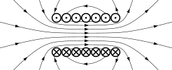
In magnetostatics

If the field is only magnetic (which is largely true in motors, for instance), some of the terms drop out, and the equation in SI units becomes:

${\displaystyle \sigma _{ij}={\frac {1}{\mu _{0}}}B_{i}B_{j}-{\frac {1}{2\mu _{0}}}B^{2}\delta _{ij}\,.}$

For cylindrical objects, such as the rotor of a motor, this is further simplified to:

${\displaystyle \sigma _{rt}={\frac {1}{\mu _{0}}}B_{r}B_{t}-{\frac {1}{2\mu _{0}}}B^{2}\delta _{rt}\,.}$

where ${\displaystyle r}$ is the shear in the radial (outward from the cylinder) direction, and ${\displaystyle t}$ is the shear in the tangential (around the cylinder) direction. It is the tangential force which spins the motor. ${\displaystyle B_{r}}$ is the flux density in the radial direction, and ${\displaystyle B_{t}}$ is the flux density in the tangential direction.

In electrostatics

In electrostatics the effects of magnetism are not present. In this case the magnetic field vanishes, i.e. ${\displaystyle \mathbf {B} =\mathbf {0} }$, and we obtain the electrostatic Maxwell stress tensor. It is given in component form by

${\displaystyle \sigma _{ij}=\varepsilon _{0}E_{i}E_{j}-{\frac {1}{2}}\varepsilon _{0}E^{2}\delta _{ij}}$

and in symbolic form by

${\displaystyle {\boldsymbol {\sigma }}=\varepsilon _{0}\mathbf {E} \otimes \mathbf {E} -{\frac {1}{2}}\varepsilon _{0}(\mathbf {E} \cdot \mathbf {E} )\mathbf {I} }$

where ${\displaystyle \mathbf {I} }$ is the appropriate identity tensor ${\displaystyle {\big (}}$usually ${\displaystyle 3\times 3{\big )}}$.

Eigenvalue

The eigenvalues of the Maxwell stress tensor are given by:

${\displaystyle \{\lambda \}=\left\{-\left({\frac {\epsilon _{0}}{2}}E^{2}+{\frac {1}{2\mu _{0}}}B^{2}\right),~\pm {\sqrt {\left({\frac {\epsilon _{0}}{2}}E^{2}-{\frac {1}{2\mu _{0}}}B^{2}\right)^{2}+{\frac {\epsilon _{0}}{\mu _{0}}}\left({\boldsymbol {E}}\cdot {\boldsymbol {B}}\right)^{2}}}\right\}}$

These eigenvalues are obtained by iteratively applying the matrix determinant lemma, in conjunction with the Sherman–Morrison formula.

Noting that the characteristic equation matrix, ${\displaystyle {\overleftrightarrow {\boldsymbol {\sigma }}}-\lambda \mathbf {\mathbb {I} } }$, can be written as

${\displaystyle {\overleftrightarrow {\boldsymbol {\sigma }}}-\lambda \mathbf {\mathbb {I} } =-\left(\lambda +V\right)\mathbf {\mathbb {I} } +\epsilon _{0}\mathbf {E} \mathbf {E} ^{\textsf {T}}+{\frac {1}{\mu _{0}}}\mathbf {B} \mathbf {B} ^{\textsf {T}}}$

where

${\displaystyle V={\frac {1}{2}}\left(\epsilon _{0}E^{2}+{\frac {1}{\mu _{0}}}B^{2}\right)}$

we set

${\displaystyle \mathbf {U} =-\left(\lambda +V\right)\mathbf {\mathbb {I} } +\epsilon _{0}\mathbf {E} \mathbf {E} ^{\textsf {T}}}$

Applying the matrix determinant lemma once, this gives us

${\displaystyle \det {\left({\overleftrightarrow {\boldsymbol {\sigma }}}-\lambda \mathbf {\mathbb {I} } \right)}=\left(1+{\frac {1}{\mu _{0}}}\mathbf {B} ^{\textsf {T}}\mathbf {U} ^{-1}\mathbf {B} \right)\det {\left(\mathbf {U} \right)}}$

Applying it again yields,

${\displaystyle \det {\left({\overleftrightarrow {\boldsymbol {\sigma }}}-\lambda \mathbf {\mathbb {I} } \right)}=\left(1+{\frac {1}{\mu _{0}}}\mathbf {B} ^{\textsf {T}}\mathbf {U} ^{-1}\mathbf {B} \right)\left(1-{\frac {\epsilon _{0}\mathbf {E} ^{\textsf {T}}\mathbf {E} }{\lambda +V}}\right)\left(-\lambda -V\right)^{3}}$

From the last multiplicand on the RHS, we immediately see that ${\displaystyle \lambda =-V}$ is one of the eigenvalues.

To find the inverse of ${\displaystyle \mathbf {U} }$, we use the Sherman-Morrison formula:

${\displaystyle \mathbf {U} ^{-1}=-\left(\lambda +V\right)^{-1}-{\frac {\epsilon _{0}\mathbf {E} \mathbf {E} ^{\textsf {T}}}{\left(\lambda +V\right)^{2}-\left(\lambda +V\right)\epsilon _{0}\mathbf {E} ^{\textsf {T}}\mathbf {E} }}}$

Factoring out a ${\displaystyle \left(-\lambda -V\right)}$ term in the determinant, we are left with finding the zeros of the rational function:

${\displaystyle \left(-\left(\lambda +V\right)-{\frac {\epsilon _{0}\left(\mathbf {E} \cdot \mathbf {B} \right)^{2}}{\mu _{0}\left(-\left(\lambda +V\right)+\epsilon _{0}\mathbf {E} ^{\textsf {T}}\mathbf {E} \right)}}\right)\left(-\left(\lambda +V\right)+\epsilon _{0}\mathbf {E} ^{\textsf {T}}\mathbf {E} \right)}$

Thus, once we solve

${\displaystyle -\left(\lambda +V\right)\left(-\left(\lambda +V\right)+\epsilon _{0}E^{2}\right)-{\frac {\epsilon _{0}}{\mu _{0}}}\left(\mathbf {E} \cdot \mathbf {B} \right)^{2}=0}$

we obtain the other two eigenvalues.

See also

• Ricci calculus
• Energy density of electric and magnetic fields
• Poynting vector
• Electromagnetic stress–energy tensor
• Magnetic pressure
• Magnetic tension

References

1. Brauer, John R. (2014-01-13). Magnetic Actuators and Sensors. John Wiley & Sons. ISBN   9781118754979.
2. Nieto-Vesperinas, Manuel; Xu, Xiaohao (12 October 2022). "The complex Maxwell stress tensor theorem: The imaginary stress tensor and the reactive strength of orbital momentum. A novel scenery underlying electromagnetic optical forces". Light: Science & Applications. 11 (1): 297. doi:10.1038/s41377-022-00979-2. PMC   9556612 . PMID   36224170.

• David J. Griffiths, "Introduction to Electrodynamics" pp. 351–352, Benjamin Cummings Inc., 2008
• John David Jackson, "Classical Electrodynamics, 3rd Ed.", John Wiley & Sons, Inc., 1999
• Richard Becker, "Electromagnetic Fields and Interactions", Dover Publications Inc., 1964