Space (mathematics)

For other uses, see Space (disambiguation).

In mathematics, a space is a set (sometimes known as a universe) endowed with a structure defining the relationships among the elements of the set. A subspace is a subset of the parent space which retains the same structure. While modern mathematics uses many types of spaces, such as Euclidean spaces, linear spaces, topological spaces, Hilbert spaces, or probability spaces, it does not define the notion of "space" itself. ^{[1] [lower-alpha 1]}

Fig. 1: Overview of types of abstract spaces. An arrow indicates is also a kind of; for instance, a normed vector space is also a metric space.

A space consists of selected mathematical objects that are treated as points, and selected relationships between these points. The nature of the points can vary widely: for example, the points can represent numbers, functions on another space, or subspaces of another space. It is the relationships that define the nature of the space. More precisely, isomorphic spaces are considered identical, where an isomorphism between two spaces is a one-to-one correspondence between their points that preserves the relationships. For example, the relationships between the points of a three-dimensional Euclidean space are uniquely determined by Euclid's axioms, ^{[lower-alpha 2]} and all three-dimensional Euclidean spaces are considered identical.

Topological notions such as continuity have natural definitions for every Euclidean space. However, topology does not distinguish straight lines from curved lines, and the relation between Euclidean and topological spaces is thus "forgetful". Relations of this kind are treated in more detail in the "Types of spaces" section.

It is not always clear whether a given mathematical object should be considered as a geometric "space", or an algebraic "structure". A general definition of "structure", proposed by Bourbaki, ^[2] embraces all common types of spaces, provides a general definition of isomorphism, and justifies the transfer of properties between isomorphic structures.

History

See also: History of geometry and Geometry § History

Table 1 | Historical development of mathematical concepts

Classic	Modern
axioms are obvious implications of definitions	axioms are conventional
theorems are absolute objective truth	theorems are implications of the corresponding axioms
relationships between points, lines etc. are determined by their nature	relationships between points, lines etc. are essential; their nature is not
mathematical objects are given to us with their structure	each mathematical theory describes its objects by some of their properties
geometry corresponds to an experimental reality	geometry is a mathematical truth
all geometric properties of the space follow from the axioms	axioms of a space need not determine all geometric properties
geometry is an autonomous and living science	classical geometry is a universal language of mathematics
space is three-dimensional	different concepts of dimension apply to different kind of spaces
space is the universe of geometry	spaces are just mathematical structures, they occur in various branches of mathematics

Before the golden age of geometry

Fig. 2: Homothety transforms a geometric figure into a similar one by scaling.

In ancient Greek mathematics, "space" was a geometric abstraction of the three-dimensional reality observed in everyday life. About 300 BC, Euclid gave axioms for the properties of space. Euclid built all of mathematics on these geometric foundations, going so far as to define numbers by comparing the lengths of line segments to the length of a chosen reference segment.

The method of coordinates (analytic geometry) was adopted by René Descartes in 1637. ^[3] At that time, geometric theorems were treated as absolute objective truths knowable through intuition and reason, similar to objects of natural science; ^{[4] : 11} and axioms were treated as obvious implications of definitions. ^{[4] : 15}

Two equivalence relations between geometric figures were used: congruence and similarity. Translations, rotations and reflections transform a figure into congruent figures; homotheties — into similar figures. For example, all circles are mutually similar, but ellipses are not similar to circles. A third equivalence relation, introduced by Gaspard Monge in 1795, occurs in projective geometry: not only ellipses, but also parabolas and hyperbolas, turn into circles under appropriate projective transformations; they all are projectively equivalent figures.

The relation between the two geometries, Euclidean and projective, ^{[4] : 133} shows that mathematical objects are not given to us with their structure. ^{[4] : 21} Rather, each mathematical theory describes its objects by some of their properties, precisely those that are put as axioms at the foundations of the theory. ^{[4] : 20}

Distances and angles cannot appear in theorems of projective geometry, since these notions are neither mentioned in the axioms of projective geometry nor defined from the notions mentioned there. The question "what is the sum of the three angles of a triangle" is meaningful in Euclidean geometry but meaningless in projective geometry.

A different situation appeared in the 19th century: in some geometries the sum of the three angles of a triangle is well-defined but different from the classical value (180 degrees). Non-Euclidean hyperbolic geometry, introduced by Nikolai Lobachevsky in 1829 and János Bolyai in 1832 (and Carl Friedrich Gauss in 1816, unpublished) ^{[4] : 133} stated that the sum depends on the triangle and is always less than 180 degrees. Eugenio Beltrami in 1868 and Felix Klein in 1871 obtained Euclidean "models" of the non-Euclidean hyperbolic geometry, and thereby completely justified this theory as a logical possibility. ^{[4] : 24  [5]}

This discovery forced the abandonment of the pretensions to the absolute truth of Euclidean geometry. It showed that axioms are not "obvious", nor "implications of definitions". Rather, they are hypotheses. To what extent do they correspond to an experimental reality? This important physical problem no longer has anything to do with mathematics. Even if a "geometry" does not correspond to an experimental reality, its theorems remain no less "mathematical truths". ^{[4] : 15}

A Euclidean model of a non-Euclidean geometry is a choice of some objects existing in Euclidean space and some relations between these objects that satisfy all axioms (and therefore, all theorems) of the non-Euclidean geometry. These Euclidean objects and relations "play" the non-Euclidean geometry like contemporary actors playing an ancient performance. Actors can imitate a situation that never occurred in reality. Relations between the actors on the stage imitate relations between the characters in the play. Likewise, the chosen relations between the chosen objects of the Euclidean model imitate the non-Euclidean relations. It shows that relations between objects are essential in mathematics, while the nature of the objects is not.

The golden age of geometry and afterwards

The word "geometry" (from Ancient Greek: geo- "earth", -metron "measurement") initially meant a practical way of processing lengths, regions and volumes in the space in which we live, but was then extended widely (as well as the notion of space in question here).

According to Bourbaki, ^{[4] : 131} the period between 1795 (Géométrie descriptive of Monge) and 1872 (the "Erlangen programme" of Klein) can be called "the golden age of geometry". The original space investigated by Euclid is now called three-dimensional Euclidean space. Its axiomatization, started by Euclid 23 centuries ago, was reformed with Hilbert's axioms, Tarski's axioms and Birkhoff's axioms. These axiom systems describe the space via primitive notions (such as "point", "between", "congruent") constrained by a number of axioms.

Analytic geometry made great progress and succeeded in replacing theorems of classical geometry with computations via invariants of transformation groups. ^{[4] : 134, 5} Since that time, new theorems of classical geometry have been of more interest to amateurs than to professional mathematicians. ^{[4] : 136} However, the heritage of classical geometry was not lost. According to Bourbaki, ^{[4] : 138} "passed over in its role as an autonomous and living science, classical geometry is thus transfigured into a universal language of contemporary mathematics".

Simultaneously, numbers began to displace geometry as the foundation of mathematics. For instance, in Richard Dedekind's 1872 essay Stetigkeit und irrationale Zahlen (Continuity and irrational numbers), he asserts that points on a line ought to have the properties of Dedekind cuts, and that therefore a line was the same thing as the set of real numbers. Dedekind is careful to note that this is an assumption that is incapable of being proven. In modern treatments, Dedekind's assertion is often taken to be the definition of a line, thereby reducing geometry to arithmetic. Three-dimensional Euclidean space is defined to be an affine space whose associated vector space of differences of its elements is equipped with an inner product. ^[6] A definition "from scratch", as in Euclid, is now not often used, since it does not reveal the relation of this space to other spaces. Also, a three-dimensional projective space is now defined as the space of all one-dimensional subspaces (that is, straight lines through the origin) of a four-dimensional vector space. This shift in foundations requires a new set of axioms, and if these axioms are adopted, the classical axioms of geometry become theorems.

A space now consists of selected mathematical objects (for instance, functions on another space, or subspaces of another space, or just elements of a set) treated as points, and selected relationships between these points. Therefore, spaces are just mathematical structures of convenience. One may expect that the structures called "spaces" are perceived more geometrically than other mathematical objects, but this is not always true.

According to the famous inaugural lecture given by Bernhard Riemann in 1854, every mathematical object parametrized by n real numbers may be treated as a point of the n-dimensional space of all such objects. ^{[4] : 140} Contemporary mathematicians follow this idea routinely and find it extremely suggestive to use the terminology of classical geometry nearly everywhere. ^{[4] : 138}

Functions are important mathematical objects. Usually they form infinite-dimensional function spaces, as noted already by Riemann ^{[4] : 141} and elaborated in the 20th century by functional analysis.

Taxonomy of spaces

Three taxonomic ranks

While each type of space has its own definition, the general idea of "space" evades formalization. Some structures are called spaces, other are not, without a formal criterion. Moreover, there is no consensus on the general idea of "structure". According to Pudlák, ^[7] "Mathematics [...] cannot be explained completely by a single concept such as the mathematical structure. Nevertheless, Bourbaki's structuralist approach is the best that we have." We will return to Bourbaki's structuralist approach in the last section "Spaces and structures", while we now outline a possible classification of spaces (and structures) in the spirit of Bourbaki.

We classify spaces on three levels. Given that each mathematical theory describes its objects by some of their properties, the first question to ask is: which properties? This leads to the first (upper) classification level. On the second level, one takes into account answers to especially important questions (among the questions that make sense according to the first level). On the third level of classification, one takes into account answers to all possible questions.

For example, the upper-level classification distinguishes between Euclidean and projective spaces, since the distance between two points is defined in Euclidean spaces but undefined in projective spaces. Another example. The question "what is the sum of the three angles of a triangle" makes sense in a Euclidean space but not in a projective space. In a non-Euclidean space the question makes sense but is answered differently, which is not an upper-level distinction.

Also, the distinction between a Euclidean plane and a Euclidean 3-dimensional space is not an upper-level distinction; the question "what is the dimension" makes sense in both cases.

The second-level classification distinguishes, for example, between Euclidean and non-Euclidean spaces; between finite-dimensional and infinite-dimensional spaces; between compact and non-compact spaces, etc. In Bourbaki's terms, ^[2] the second-level classification is the classification by "species". Unlike biological taxonomy, a space may belong to several species.

The third-level classification distinguishes, for example, between spaces of different dimension, but does not distinguish between a plane of a three-dimensional Euclidean space, treated as a two-dimensional Euclidean space, and the set of all pairs of real numbers, also treated as a two-dimensional Euclidean space. Likewise it does not distinguish between different Euclidean models of the same non-Euclidean space. More formally, the third level classifies spaces up to isomorphism. An isomorphism between two spaces is defined as a one-to-one correspondence between the points of the first space and the points of the second space, that preserves all relations stipulated according to the first level. Mutually isomorphic spaces are thought of as copies of a single space. If one of them belongs to a given species then they all do.

The notion of isomorphism sheds light on the upper-level classification. Given a one-to-one correspondence between two spaces of the same upper-level class, one may ask whether it is an isomorphism or not. This question makes no sense for two spaces of different classes.

An isomorphism to itself is called an automorphism. Automorphisms of a Euclidean space are shifts, rotations, reflections and compositions of these. Euclidean space is homogeneous in the sense that every point can be transformed into every other point by some automorphism.

Euclidean axioms ^{[lower-alpha 2]} leave no freedom; they determine uniquely all geometric properties of the space. More exactly: all three-dimensional Euclidean spaces are mutually isomorphic. In this sense we have "the" three-dimensional Euclidean space. In Bourbaki's terms, the corresponding theory is univalent. In contrast, topological spaces are generally non-isomorphic; their theory is multivalent. A similar idea occurs in mathematical logic: a theory is called categorical if all its models of the same cardinality are mutually isomorphic. According to Bourbaki, ^[8] the study of multivalent theories is the most striking feature which distinguishes modern mathematics from classical mathematics.

Relations between species of spaces

Topological notions (continuity, convergence, open sets, closed sets etc.) are defined naturally in every Euclidean space. In other words, every Euclidean space is also a topological space. Every isomorphism between two Euclidean spaces is also an isomorphism between the corresponding topological spaces (called "homeomorphism"), but the converse is wrong: a homeomorphism may distort distances. In Bourbaki's terms, ^[2] "topological space" is an underlying structure of the "Euclidean space" structure. Similar ideas occur in category theory: the category of Euclidean spaces is a concrete category over the category of topological spaces; the forgetful (or "stripping") functor maps the former category to the latter category.

A three-dimensional Euclidean space is a special case of a Euclidean space. In Bourbaki's terms, ^[2] the species of three-dimensional Euclidean space is richer than the species of Euclidean space. Likewise, the species of compact topological space is richer than the species of topological space.

Fig. 3: Example relations between species of spaces

Such relations between species of spaces may be expressed diagrammatically as shown in Fig. 3. An arrow from A to B means that every A-space is also a B-space, or may be treated as a B-space, or provides a B-space, etc. Treating A and B as classes of spaces one may interpret the arrow as a transition from A to B. (In Bourbaki's terms, ^[9] "procedure of deduction" of a B-space from a A-space. Not quite a function unless the classes A,B are sets; this nuance does not invalidate the following.) The two arrows on Fig. 3 are not invertible, but for different reasons.

The transition from "Euclidean" to "topological" is forgetful. Topology distinguishes continuous from discontinuous, but does not distinguish rectilinear from curvilinear. Intuition tells us that the Euclidean structure cannot be restored from the topology. A proof uses an automorphism of the topological space (that is, self-homeomorphism) that is not an automorphism of the Euclidean space (that is, not a composition of shifts, rotations and reflections). Such transformation turns the given Euclidean structure into a (isomorphic but) different Euclidean structure; both Euclidean structures correspond to a single topological structure.

In contrast, the transition from "3-dim Euclidean" to "Euclidean" is not forgetful; a Euclidean space need not be 3-dimensional, but if it happens to be 3-dimensional, it is full-fledged, no structure is lost. In other words, the latter transition is injective (one-to-one), while the former transition is not injective (many-to-one). We denote injective transitions by an arrow with a barbed tail, "↣" rather than "→".

Both transitions are not surjective, that is, not every B-space results from some A-space. First, a 3-dim Euclidean space is a special (not general) case of a Euclidean space. Second, a topology of a Euclidean space is a special case of topology (for instance, it must be non-compact, and connected, etc). We denote surjective transitions by a two-headed arrow, "↠" rather than "→". See for example Fig. 4; there, the arrow from "real linear topological" to "real linear" is two-headed, since every real linear space admits some (at least one) topology compatible with its linear structure.

Such topology is non-unique in general, but unique when the real linear space is finite-dimensional. For these spaces the transition is both injective and surjective, that is, bijective; see the arrow from "finite-dim real linear topological" to "finite-dim real linear" on Fig. 4. The inverse transition exists (and could be shown by a second, backward arrow). The two species of structures are thus equivalent. In practice, one makes no distinction between equivalent species of structures. ^[10] Equivalent structures may be treated as a single structure, as shown by a large box on Fig. 4.

The transitions denoted by the arrows obey isomorphisms. That is, two isomorphic A-spaces lead to two isomorphic B-spaces.

The diagram on Fig. 4 is commutative. That is, all directed paths in the diagram with the same start and endpoints lead to the same result. Other diagrams below are also commutative, except for dashed arrows on Fig. 9. The arrow from "topological" to "measurable" is dashed for the reason explained there: "In order to turn a topological space into a measurable space one endows it with a σ-algebra. The σ-algebra of Borel sets is the most popular, but not the only choice." A solid arrow denotes a prevalent, so-called "canonical" transition that suggests itself naturally and is widely used, often implicitly, by default. For example, speaking about a continuous function on a Euclidean space, one need not specify its topology explicitly. In fact, alternative topologies exist and are used sometimes, for example, the fine topology; but these are always specified explicitly, since they are much less notable that the prevalent topology. A dashed arrow indicates that several transitions are in use and no one is quite prevalent.

Types of spaces

Linear and topological spaces

Fig. 4: Relations between mathematical spaces: linear, topological etc

Two basic spaces are linear spaces (also called vector spaces) and topological spaces.

Linear spaces are of algebraic nature; there are real linear spaces (over the field of real numbers), complex linear spaces (over the field of complex numbers), and more generally, linear spaces over any field. Every complex linear space is also a real linear space (the latter underlies the former), since each complex number can be specified by two real numbers. For example, the complex plane treated as a one-dimensional complex linear space may be downgraded to a two-dimensional real linear space. In contrast, the real line can be treated as a one-dimensional real linear space but not a complex linear space. See also field extensions. More generally, a vector space over a field also has the structure of a vector space over a subfield of that field. Linear operations, given in a linear space by definition, lead to such notions as straight lines (and planes, and other linear subspaces); parallel lines; ellipses (and ellipsoids). However, it is impossible to define orthogonal (perpendicular) lines, or to single out circles among ellipses, because in a linear space there is no structure like a scalar product that could be used for measuring angles. The dimension of a linear space is defined as the maximal number of linearly independent vectors or, equivalently, as the minimal number of vectors that span the space; it may be finite or infinite. Two linear spaces over the same field are isomorphic if and only if they are of the same dimension. A n-dimensional complex linear space is also a 2n-dimensional real linear space.

Topological spaces are of analytic nature. Open sets, given in a topological space by definition, lead to such notions as continuous functions, paths, maps; convergent sequences, limits; interior, boundary, exterior. However, uniform continuity, bounded sets, Cauchy sequences, differentiable functions (paths, maps) remain undefined. Isomorphisms between topological spaces are traditionally called homeomorphisms; these are one-to-one correspondences continuous in both directions. The open interval (0,1) is homeomorphic to the whole real line (−∞,∞) but not homeomorphic to the closed interval [0,1], nor to a circle. The surface of a cube is homeomorphic to a sphere (the surface of a ball) but not homeomorphic to a torus. Euclidean spaces of different dimensions are not homeomorphic, which seems evident, but is not easy to prove. The dimension of a topological space is difficult to define; inductive dimension (based on the observation that the dimension of the boundary of a geometric figure is usually one less than the dimension of the figure itself) and Lebesgue covering dimension can be used. In the case of a n-dimensional Euclidean space, both topological dimensions are equal to n.

Every subset of a topological space is itself a topological space (in contrast, only linear subsets of a linear space are linear spaces). Arbitrary topological spaces, investigated by general topology (called also point-set topology) are too diverse for a complete classification up to homeomorphism. Compact topological spaces are an important class of topological spaces ("species" of this "type"). Every continuous function is bounded on such space. The closed interval [0,1] and the extended real line [−∞,∞] are compact; the open interval (0,1) and the line (−∞,∞) are not. Geometric topology investigates manifolds (another "species" of this "type"); these are topological spaces locally homeomorphic to Euclidean spaces (and satisfying a few extra conditions). Low-dimensional manifolds are completely classified up to homeomorphism.

Both the linear and topological structures underlie the linear topological space (in other words, topological vector space) structure. A linear topological space is both a real or complex linear space and a topological space, such that the linear operations are continuous. So a linear space that is also topological is not in general a linear topological space.

Every finite-dimensional real or complex linear space is a linear topological space in the sense that it carries one and only one topology that makes it a linear topological space. The two structures, "finite-dimensional real or complex linear space" and "finite-dimensional linear topological space", are thus equivalent, that is, mutually underlying. Accordingly, every invertible linear transformation of a finite-dimensional linear topological space is a homeomorphism. The three notions of dimension (one algebraic and two topological) agree for finite-dimensional real linear spaces. In infinite-dimensional spaces, however, different topologies can conform to a given linear structure, and invertible linear transformations are generally not homeomorphisms.

Affine and projective spaces

Fig. 5: Relations between mathematical spaces: affine, projective etc

It is convenient to introduce affine and projective spaces by means of linear spaces, as follows. A n-dimensional linear subspace of a (n+1)-dimensional linear space, being itself a n-dimensional linear space, is not homogeneous; it contains a special point, the origin. Shifting it by a vector external to it, one obtains a n-dimensional affine subspace. It is homogeneous. An affine space need not be included into a linear space, but is isomorphic to an affine subspace of a linear space. All n-dimensional affine spaces over a given field are mutually isomorphic. In the words of John Baez, "an affine space is a vector space that's forgotten its origin". In particular, every linear space is also an affine space.

Given an n-dimensional affine subspace A in a (n+1)-dimensional linear space L, a straight line in A may be defined as the intersection of A with a two-dimensional linear subspace of L that intersects A: in other words, with a plane through the origin that is not parallel to A. More generally, a k-dimensional affine subspace of A is the intersection of A with a (k+1)-dimensional linear subspace of L that intersects A.

Every point of the affine subspace A is the intersection of A with a one-dimensional linear subspace of L. However, some one-dimensional subspaces of L are parallel to A; in some sense, they intersect A at infinity. The set of all one-dimensional linear subspaces of a (n+1)-dimensional linear space is, by definition, a n-dimensional projective space. And the affine subspace A is embedded into the projective space as a proper subset. However, the projective space itself is homogeneous. A straight line in the projective space corresponds to a two-dimensional linear subspace of the (n+1)-dimensional linear space. More generally, a k-dimensional projective subspace of the projective space corresponds to a (k+1)-dimensional linear subspace of the (n+1)-dimensional linear space, and is isomorphic to the k-dimensional projective space.

Defined this way, affine and projective spaces are of algebraic nature; they can be real, complex, and more generally, over any field.

Every real or complex affine or projective space is also a topological space. An affine space is a non-compact manifold; a projective space is a compact manifold. In a real projective space a straight line is homeomorphic to a circle, therefore compact, in contrast to a straight line in a linear of affine space.

Metric and uniform spaces

Fig. 6: Relations between mathematical spaces: metric, uniform etc

Distances between points are defined in a metric space. Isomorphisms between metric spaces are called isometries. Every metric space is also a topological space. A topological space is called metrizable, if it underlies a metric space. All manifolds are metrizable.

In a metric space, we can define bounded sets and Cauchy sequences. A metric space is called complete if all Cauchy sequences converge. Every incomplete space is isometrically embedded, as a dense subset, into a complete space (the completion). Every compact metric space is complete; the real line is non-compact but complete; the open interval (0,1) is incomplete.

Every Euclidean space is also a complete metric space. Moreover, all geometric notions immanent to a Euclidean space can be characterized in terms of its metric. For example, the straight segment connecting two given points A and C consists of all points B such that the distance between A and C is equal to the sum of two distances, between A and B and between B and C.

The Hausdorff dimension (related to the number of small balls that cover the given set) applies to metric spaces, and can be non-integer (especially for fractals). For a n-dimensional Euclidean space, the Hausdorff dimension is equal to n.

Uniform spaces do not introduce distances, but still allow one to use uniform continuity, Cauchy sequences (or filters or nets), completeness and completion. Every uniform space is also a topological space. Every linear topological space (metrizable or not) is also a uniform space, and is complete in finite dimension but generally incomplete in infinite dimension. More generally, every commutative topological group is also a uniform space. A non-commutative topological group, however, carries two uniform structures, one left-invariant, the other right-invariant.

Normed, Banach, inner product, and Hilbert spaces

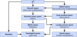
Fig. 7: Relations between mathematical spaces: normed, Banach etc

Vectors in a Euclidean space form a linear space, but each vector ${\displaystyle x}$ has also a length, in other words, norm, ${\displaystyle \lVert x\rVert }$. A real or complex linear space endowed with a norm is a normed space. Every normed space is both a linear topological space and a metric space. A Banach space is a complete normed space. Many spaces of sequences or functions are infinite-dimensional Banach spaces.

The set of all vectors of norm less than one is called the unit ball of a normed space. It is a convex, centrally symmetric set, generally not an ellipsoid; for example, it may be a polygon (in the plane) or, more generally, a polytope (in arbitrary finite dimension). The parallelogram law (called also parallelogram identity)

${\displaystyle \lVert x-y\rVert ^{2}+\lVert x+y\rVert ^{2}=2\lVert x\rVert ^{2}+2\lVert y\rVert ^{2}\ ,}$

generally fails in normed spaces, but holds for vectors in Euclidean spaces, which follows from the fact that the squared Euclidean norm of a vector is its inner product with itself, ${\displaystyle \lVert x\rVert ^{2}=(x,x)}$.

An inner product space is a real or complex linear space, endowed with a bilinear or respectively sesquilinear form, satisfying some conditions and called an inner product. Every inner product space is also a normed space. A normed space underlies an inner product space if and only if it satisfies the parallelogram law, or equivalently, if its unit ball is an ellipsoid. Angles between vectors are defined in inner product spaces. A Hilbert space is defined as a complete inner product space. (Some authors insist that it must be complex, others admit also real Hilbert spaces.) Many spaces of sequences or functions are infinite-dimensional Hilbert spaces. Hilbert spaces are very important for quantum theory. ^[11]

All n-dimensional real inner product spaces are mutually isomorphic. One may say that the n-dimensional Euclidean space is the n-dimensional real inner product space that forgot its origin.

Smooth and Riemannian manifolds

Fig. 8: Relations between mathematical spaces: smooth, Riemannian etc

Smooth manifolds are not called "spaces", but could be. Every smooth manifold is a topological manifold, and can be embedded into a finite-dimensional linear space. Smooth surfaces in a finite-dimensional linear space are smooth manifolds: for example, the surface of an ellipsoid is a smooth manifold, a polytope is not. Real or complex finite-dimensional linear, affine and projective spaces are also smooth manifolds.

At each one of its points, a smooth path in a smooth manifold has a tangent vector that belongs to the manifold's tangent space at this point. Tangent spaces to an n-dimensional smooth manifold are n-dimensional linear spaces. The differential of a smooth function on a smooth manifold provides a linear functional on the tangent space at each point.

A Riemannian manifold, or Riemann space, is a smooth manifold whose tangent spaces are endowed with inner products satisfying some conditions. Euclidean spaces are also Riemann spaces. Smooth surfaces in Euclidean spaces are Riemann spaces. A hyperbolic non-Euclidean space is also a Riemann space. A curve in a Riemann space has a length, and the length of the shortest curve between two points defines a distance, such that the Riemann space is a metric space. The angle between two curves intersecting at a point is the angle between their tangent lines.

Waiving positivity of inner products on tangent spaces, one obtains pseudo-Riemann spaces, including the Lorentzian spaces that are very important for general relativity.

Measurable, measure, and probability spaces

Fig. 9: Relations between mathematical spaces: measurable, measure etc

Waiving distances and angles while retaining volumes (of geometric bodies) one reaches measure theory. Besides the volume, a measure generalizes the notions of area, length, mass (or charge) distribution, and also probability distribution, according to Andrey Kolmogorov's approach to probability theory.

A "geometric body" of classical mathematics is much more regular than just a set of points. The boundary of the body is of zero volume. Thus, the volume of the body is the volume of its interior, and the interior can be exhausted by an infinite sequence of cubes. In contrast, the boundary of an arbitrary set of points can be of non-zero volume (an example: the set of all rational points inside a given cube). Measure theory succeeded in extending the notion of volume to a vast class of sets, the so-called measurable sets. Indeed, non-measurable sets almost never occur in applications.

Measurable sets, given in a measurable space by definition, lead to measurable functions and maps. In order to turn a topological space into a measurable space one endows it with a σ-algebra. The σ-algebra of Borel sets is the most popular, but not the only choice. (Baire sets, universally measurable sets, etc, are also used sometimes.) The topology is not uniquely determined by the Borel σ-algebra; for example, the norm topology and the weak topology on a separable Hilbert space lead to the same Borel σ-algebra. Not every σ-algebra is the Borel σ-algebra of some topology. ^{[lower-alpha 3]} Actually, a σ-algebra can be generated by a given collection of sets (or functions) irrespective of any topology. Every subset of a measurable space is itself a measurable space.

Standard measurable spaces (also called standard Borel spaces) are especially useful due to some similarity to compact spaces (see EoM). Every bijective measurable mapping between standard measurable spaces is an isomorphism; that is, the inverse mapping is also measurable. And a mapping between such spaces is measurable if and only if its graph is measurable in the product space. Similarly, every bijective continuous mapping between compact metric spaces is a homeomorphism; that is, the inverse mapping is also continuous. And a mapping between such spaces is continuous if and only if its graph is closed in the product space.

Every Borel set in a Euclidean space (and more generally, in a complete separable metric space), endowed with the Borel σ-algebra, is a standard measurable space. All uncountable standard measurable spaces are mutually isomorphic.

A measure space is a measurable space endowed with a measure. A Euclidean space with the Lebesgue measure is a measure space. Integration theory defines integrability and integrals of measurable functions on a measure space.

Sets of measure 0, called null sets, are negligible. Accordingly, a "mod 0 isomorphism" is defined as isomorphism between subsets of full measure (that is, with negligible complement).

A probability space is a measure space such that the measure of the whole space is equal to 1. The product of any family (finite or not) of probability spaces is a probability space. In contrast, for measure spaces in general, only the product of finitely many spaces is defined. Accordingly, there are many infinite-dimensional probability measures (especially, Gaussian measures), but no infinite-dimensional Lebesgue measures.

Standard probability spaces are especially useful. On a standard probability space a conditional expectation may be treated as the integral over the conditional measure (regular conditional probabilities, see also disintegration of measure). Given two standard probability spaces, every homomorphism of their measure algebras is induced by some measure preserving map. Every probability measure on a standard measurable space leads to a standard probability space. The product of a sequence (finite or not) of standard probability spaces is a standard probability space. All non-atomic standard probability spaces are mutually isomorphic mod 0; one of them is the interval (0,1) with the Lebesgue measure.

These spaces are less geometric. In particular, the idea of dimension, applicable (in one form or another) to all other spaces, does not apply to measurable, measure and probability spaces.

Non-commutative geometry

The theoretical study of calculus, known as mathematical analysis, led in the early 20th century to the consideration of linear spaces of real-valued or complex-valued functions. The earliest examples of these were function spaces, each one adapted to its own class of problems. These examples shared many common features, and these features were soon abstracted into Hilbert spaces, Banach spaces, and more general topological vector spaces. These were a powerful toolkit for the solution of a wide range of mathematical problems.

The most detailed information was carried by a class of spaces called Banach algebras. These are Banach spaces together with a continuous multiplication operation. An important early example was the Banach algebra of essentially bounded measurable functions on a measure space X. This set of functions is a Banach space under pointwise addition and scalar multiplication. With the operation of pointwise multiplication, it becomes a special type of Banach space, one now called a commutative von Neumann algebra. Pointwise multiplication determines a representation of this algebra on the Hilbert space of square integrable functions on X. An early observation of John von Neumann was that this correspondence also worked in reverse: Given some mild technical hypotheses, a commutative von Neumann algebra together with a representation on a Hilbert space determines a measure space, and these two constructions (of a von Neumann algebra plus a representation and of a measure space) are mutually inverse.

Von Neumann then proposed that non-commutative von Neumann algebras should have geometric meaning, just as commutative von Neumann algebras do. Together with Francis Murray, he produced a classification of von Neumann algebras. The direct integral construction shows how to break any von Neumann algebra into a collection of simpler algebras called factors. Von Neumann and Murray classified factors into three types. Type I was nearly identical to the commutative case. Types II and III exhibited new phenomena. A type II von Neumann algebra determined a geometry with the peculiar feature that the dimension could be any non-negative real number, not just an integer. Type III algebras were those that were neither types I nor II, and after several decades of effort, these were proven to be closely related to type II factors.

A slightly different approach to the geometry of function spaces developed at the same time as von Neumann and Murray's work on the classification of factors. This approach is the theory of C*-algebras. Here, the motivating example is the C*-algebra${\displaystyle C_{0}(X)}$, where X is a locally compact Hausdorff topological space. By definition, this is the algebra of continuous complex-valued functions on X that vanish at infinity (which loosely means that the farther you go from a chosen point, the closer the function gets to zero) with the operations of pointwise addition and multiplication. The Gelfand–Naimark theorem implied that there is a correspondence between commutative C*-algebras and geometric objects: Every commutative C*-algebra is of the form ${\displaystyle C_{0}(X)}$ for some locally compact Hausdorff space X. Consequently it is possible to study locally compact Hausdorff spaces purely in terms of commutative C*-algebras. Non-commutative geometry takes this as inspiration for the study of non-commutative C*-algebras: If there were such a thing as a "non-commutative space X," then its ${\displaystyle C_{0}(X)}$ would be a non-commutative C*-algebra; if in addition the Gelfand–Naimark theorem applied to these non-existent objects, then spaces (commutative or not) would be the same as C*-algebras; so, for lack of a direct approach to the definition of a non-commutative space, a non-commutative space is defined to be a non-commutative C*-algebra. Many standard geometric tools can be restated in terms of C*-algebras, and this gives geometrically-inspired techniques for studying non-commutative C*-algebras.

Both of these examples are now cases of a field called non-commutative geometry. The specific examples of von Neumann algebras and C*-algebras are known as non-commutative measure theory and non-commutative topology, respectively. Non-commutative geometry is not merely a pursuit of generality for its own sake and is not just a curiosity. Non-commutative spaces arise naturally, even inevitably, from some constructions. For example, consider the non-periodic Penrose tilings of the plane by kites and darts. It is a theorem that, in such a tiling, every finite patch of kites and darts appears infinitely often. As a consequence, there is no way to distinguish two Penrose tilings by looking at a finite portion. This makes it impossible to assign the set of all tilings a topology in the traditional sense. Despite this, the Penrose tilings determine a non-commutative C*-algebra, and consequently they can be studied by the techniques of non-commutative geometry. Another example, and one of great interest within differential geometry, comes from foliations of manifolds. These are ways of splitting the manifold up into smaller-dimensional submanifolds called leaves, each of which is locally parallel to others nearby. The set of all leaves can be made into a topological space. However, the example of an irrational rotation shows that this topological space can be inaccessible to the techniques of classical measure theory. However, there is a non-commutative von Neumann algebra associated to the leaf space of a foliation, and once again, this gives an otherwise unintelligible space a good geometric structure.

Schemes

Fig. 10: Relations between mathematical spaces: schemes, stacks etc

Algebraic geometry studies the geometric properties of polynomial equations. Polynomials are a type of function defined from the basic arithmetic operations of addition and multiplication. Because of this, they are closely tied to algebra. Algebraic geometry offers a way to apply geometric techniques to questions of pure algebra, and vice versa.

Prior to the 1940s, algebraic geometry worked exclusively over the complex numbers, and the most fundamental variety was projective space. The geometry of projective space is closely related to the theory of perspective, and its algebra is described by homogeneous polynomials. All other varieties were defined as subsets of projective space. Projective varieties were subsets defined by a set of homogeneous polynomials. At each point of the projective variety, all the polynomials in the set were required to equal zero. The complement of the zero set of a linear polynomial is an affine space, and an affine variety was the intersection of a projective variety with an affine space.

André Weil saw that geometric reasoning could sometimes be applied in number-theoretic situations where the spaces in question might be discrete or even finite. In pursuit of this idea, Weil rewrote the foundations of algebraic geometry, both freeing algebraic geometry from its reliance on complex numbers and introducing abstract algebraic varieties which were not embedded in projective space. These are now simply called varieties.

The type of space that underlies most modern algebraic geometry is even more general than Weil's abstract algebraic varieties. It was introduced by Alexander Grothendieck and is called a scheme. One of the motivations for scheme theory is that polynomials are unusually structured among functions, and algebraic varieties are consequently rigid. This presents problems when attempting to study degenerate situations. For example, almost any pair of points on a circle determines a unique line called the secant line, and as the two points move around the circle, the secant line varies continuously. However, when the two points collide, the secant line degenerates to a tangent line. The tangent line is unique, but the geometry of this configuration—a single point on a circle—is not expressive enough to determine a unique line. Studying situations like this requires a theory capable of assigning extra data to degenerate situations.

One of the building blocks of a scheme is a topological space. Topological spaces have continuous functions, but continuous functions are too general to reflect the underlying algebraic structure of interest. The other ingredient in a scheme, therefore, is a sheaf on the topological space, called the "structure sheaf". On each open subset of the topological space, the sheaf specifies a collection of functions, called "regular functions". The topological space and the structure sheaf together are required to satisfy conditions that mean the functions come from algebraic operations.

Like manifolds, schemes are defined as spaces that are locally modeled on a familiar space. In the case of manifolds, the familiar space is Euclidean space. For a scheme, the local models are called affine schemes. Affine schemes provide a direct link between algebraic geometry and commutative algebra. The fundamental objects of study in commutative algebra are commutative rings. If ${\displaystyle R}$ is a commutative ring, then there is a corresponding affine scheme ${\displaystyle \operatorname {Spec} R}$ which translates the algebraic structure of ${\displaystyle R}$ into geometry. Conversely, every affine scheme determines a commutative ring, namely, the ring of global sections of its structure sheaf. These two operations are mutually inverse, so affine schemes provide a new language with which to study questions in commutative algebra. By definition, every point in a scheme has an open neighborhood which is an affine scheme.

There are many schemes that are not affine. In particular, projective spaces satisfy a condition called properness which is analogous to compactness. Affine schemes cannot be proper (except in trivial situations like when the scheme has only a single point), and hence no projective space is an affine scheme (except for zero-dimensional projective spaces). Projective schemes, meaning those that arise as closed subschemes of a projective space, are the single most important family of schemes. ^[12]

Several generalizations of schemes have been introduced. Michael Artin defined an algebraic space as the quotient of a scheme by the equivalence relations that define étale morphisms. Algebraic spaces retain many of the useful properties of schemes while simultaneously being more flexible. For instance, the Keel–Mori theorem can be used to show that many moduli spaces are algebraic spaces.

More general than an algebraic space is a Deligne–Mumford stack. DM stacks are similar to schemes, but they permit singularities that cannot be described solely in terms of polynomials. They play the same role for schemes that orbifolds do for manifolds. For example, the quotient of the affine plane by a finite group of rotations around the origin yields a Deligne–Mumford stack that is not a scheme or an algebraic space. Away from the origin, the quotient by the group action identifies finite sets of equally spaced points on a circle. But at the origin, the circle consists of only a single point, the origin itself, and the group action fixes this point. In the quotient DM stack, however, this point comes with the extra data of being a quotient. This kind of refined structure is useful in the theory of moduli spaces, and in fact, it was originally introduced to describe moduli of algebraic curves.

A further generalization are the algebraic stacks, also called Artin stacks. DM stacks are limited to quotients by finite group actions. While this suffices for many problems in moduli theory, it is too restrictive for others, and Artin stacks permit more general quotients.

Topoi

Fig. 11: Relations between mathematical spaces: locales, topoi etc

In Grothendieck's work on the Weil conjectures, he introduced a new type of topology now called a Grothendieck topology. A topological space (in the ordinary sense) axiomatizes the notion of "nearness," making two points be nearby if and only if they lie in many of the same open sets. By contrast, a Grothendieck topology axiomatizes the notion of "covering". A covering of a space is a collection of subspaces that jointly contain all the information of the ambient space. Since sheaves are defined in terms of coverings, a Grothendieck topology can also be seen as an axiomatization of the theory of sheaves.

Grothendieck's work on his topologies led him to the theory of topoi. In his memoir Récoltes et Semailles, he called them his "most vast conception". ^[13] A sheaf (either on a topological space or with respect to a Grothendieck topology) is used to express local data. The category of all sheaves carries all possible ways of expressing local data. Since topological spaces are constructed from points, which are themselves a kind of local data, the category of sheaves can therefore be used as a replacement for the original space. Grothendieck consequently defined a topos to be a category of sheaves and studied topoi as objects of interest in their own right. These are now called Grothendieck topoi.

Every topological space determines a topos, and vice versa. There are topological spaces where taking the associated topos loses information, but these are generally considered pathological. (A necessary and sufficient condition is that the topological space be a sober space.) Conversely, there are topoi whose associated topological spaces do not capture the original topos. But, far from being pathological, these topoi can be of great mathematical interest. For instance, Grothendieck's theory of étale cohomology (which eventually led to the proof of the Weil conjectures) can be phrased as cohomology in the étale topos of a scheme, and this topos does not come from a topological space.

Topological spaces in fact lead to very special topoi called locales. The set of open subsets of a topological space determines a lattice. The axioms for a topological space cause these lattices to be complete Heyting algebras. The theory of locales takes this as its starting point. A locale is defined to be a complete Heyting algebra, and the elementary properties of topological spaces are re-expressed and reproved in these terms. The concept of a locale turns out to be more general than a topological space, in that every sober topological space determines a unique locale, but many interesting locales do not come from topological spaces. Because locales need not have points, the study of locales is somewhat jokingly called pointless topology.

Topoi also display deep connections to mathematical logic. Every Grothendieck topos has a special sheaf called a subobject classifier. This subobject classifier functions like the set of all possible truth values. In the topos of sets, the subobject classifier is the set ${\displaystyle \{0,1\}}$, corresponding to "False" and "True". But in other topoi, the subobject classifier can be much more complicated. Lawvere and Tierney recognized that axiomatizing the subobject classifier yielded a more general kind of topos, now known as an elementary topos, and that elementary topoi were models of intuitionistic logic. In addition to providing a powerful way to apply tools from logic to geometry, this made possible the use of geometric methods in logic.

Spaces and structure

According to Kevin Arlin,

Neither of these words ["space" and "structure"] have a single mathematical definition. The English words can be used in essentially all the same situations, but you often think of a "space" as more geometric and a "structure" as more algebraic. [...] So you could think of "structures" as places we do algebra, and "spaces" as places we do geometry. Then a lot of great mathematics has come from passing from structures to spaces and vice versa, as when we look at the fundamental group of a topological space or the spectrum of a ring. But in the end, the distinction is neither hard nor fast and only goes so far: many things are obviously both structures and spaces, some things are not obviously either, and some people might well disagree with everything I've said here. ^[1]

Nevertheless, a general definition of "structure" was proposed by Bourbaki; ^[2] it embraces all types of spaces mentioned above, (nearly?) all types of mathematical structures used till now, and more. It provides a general definition of isomorphism, and justifies transfer of properties between isomorphic structures. However, it was never used actively in mathematical practice (not even in the mathematical treatises written by Bourbaki himself). Here are the last phrases from a review by Robert Reed ^[14] of a book by Leo Corry:

Corry does not seem to feel that any formal definition of structure could do justice to the use of the concept in actual mathematical practice [...] Corry's view could be summarized as the belief that 'structure' refers essentially to a way of doing mathematics, and is therefore a concept probably just as far from being precisely definable as the cultural artifact of mathematics itself.

For more information on mathematical structures see Wikipedia: mathematical structure, equivalent definitions of mathematical structures, and transport of structure.

The distinction between geometric "spaces" and algebraic "structures" is sometimes clear, sometimes elusive. Clearly, groups are algebraic, while Euclidean spaces are geometric. Modules over rings are as algebraic as groups. In particular, when the ring appears to be a field, the module appears to be a linear space; is it algebraic or geometric? In particular, when it is finite-dimensional, over real numbers, and endowed with inner product, it becomes Euclidean space; now geometric. The (algebraic?) field of real numbers is the same as the (geometric?) real line. Its algebraic closure, the (algebraic?) field of complex numbers, is the same as the (geometric?) complex plane. It is first of all "a place we do analysis" (rather than algebra or geometry).

Every space treated in Section "Types of spaces" above, except for "Non-commutative geometry", "Schemes" and "Topoi" subsections, is a set (the "principal base set" of the structure, according to Bourbaki) endowed with some additional structure; elements of the base set are usually called "points" of this space. In contrast, elements of (the base set of) an algebraic structure usually are not called "points".

However, sometimes one uses more than one principal base set. For example, two-dimensional projective geometry may be formalized via two base sets, the set of points and the set of lines. Moreover, a striking feature of projective planes is the symmetry of the roles played by points and lines. A less geometric example: a graph may be formalized via two base sets, the set of vertices (called also nodes or points) and the set of edges (called also arcs or lines). Generally, finitely many principal base sets and finitely many auxiliary base sets are stipulated by Bourbaki.

Many mathematical structures of geometric flavor treated in the "Non-commutative geometry", "Schemes" and "Topoi" subsections above do not stipulate a base set of points. For example, "pointless topology" (in other words, point-free topology, or locale theory) starts with a single base set whose elements imitate open sets in a topological space (but are not sets of points); see also mereotopology and point-free geometry.

List of mathematical spaces

Main category: Space (mathematics)

• Affine space
• Algebraic space
• Baire space
• Banach space
• Base space
• Bergman space
• Berkovich space
• Besov space
• Borel space
• Calabi-Yau space
• Cantor space
• Cauchy space
• Cellular space
• Chu space
• Closure space
• Conformal space
• Complex analytic space
• Drinfeld's symmetric space
• Eilenberg–Mac Lane space
• Euclidean space
• Fiber space
• Finsler space
• First-countable space
• Fréchet space
• Function space
• G-space
• Geometric space
• Green space (topological space)
• Hardy space
• Hausdorff space
• Heisenberg space
• Hilbert space
• Homogeneous space
• Inner product space
• Kolmogorov space
• L^p-space
• Lens space
• Liouville space
• Locally finite space
• Loop space
• Lorentz space
• Mapping space
• Measure space
• Metric space
• Minkowski space
• Müntz space
• Normed space
• Paracompact space
• Perfectoid space
• Planar space
• Polish space
• Probability space
• Projective space
• Proximity space
• Quadratic space
• Quotient space (disambiguation)
• Riemann's Moduli space
• Sample space
• Sequence space
• Sierpiński space
• Sobolev space
• Standard space
• State space
• Stone space
• Symplectic space (disambiguation)
• T₂ space
• Teichmüller space
• Tensor space
• Topological space
• Topological vector space
• Total space
• Uniform space
• Vector space

See also

• Dimension#In mathematics
• Mathematical structure
• Transport of structure
• Set (mathematics)
• Category (mathematics)

Notes

1. Similarly, several types of numbers are in use (natural, integral, rational, real, complex); each one has its own definition; but just "number" is not used as a mathematical notion and has no definition.
2. Reformed by Hilbert, Tarski and Birkhoff in order to avoid hidden assumptions found in Euclid's Elements.
3. The space ${\displaystyle 2^{\mathbb {R} }}$ (equipped with its tensor product σ-algebra) has a measurable structure which is not generated by a topology. A proof can be found in this answer on MathOverflow .

Footnotes

1. Carlson, Kevin (August 2, 2012). "Difference between 'space' and 'mathematical structure'?". Stack Exchange.
2. Bourbaki 1968 , Chapter IV
3. Itô 1993 , page 987
4. Bourbaki, Nicolas (1994). Elements of the history of mathematics . Masson (original), Springer (translation). doi:10.1007/978-3-642-61693-8. ISBN   978-3-540-64767-6.
5. Gray, Jeremy (1989). Ideas of Space: Euclidean, Non-Euclidean and Relativistic (second ed.). Clarendon Press. ISBN   978-0198539353.
6. Gallier, Jean (2011). "Basics of Euclidean Geometry". Geometric Methods and Applications. Texts in Applied Mathematics. Vol. 38. Springer. pp. 177–212. doi:10.1007/978-1-4419-9961-0_6. ISBN   978-1-4419-9960-3. See also OpenCourseWare.
7. Pudlák, Pavel (2013). Logical Foundations of Mathematics and Computational Complexity: A Gentle Introduction. Springer Monographs in Mathematics. Springer. doi:10.1007/978-3-319-00119-7. ISBN   978-3-319-00118-0.
8. Bourbaki 1968 , page 385
9. Bourbaki 1968 , Sect.IV.1.6
10. Bourbaki 1968 , Sect.IV.1.7
11. Lanczos, Cornelius (1970). Space through the Ages: The Evolution of Geometrical Ideas from Pythagoras to Hilbert and Einstein . Academic Press. p.  269. ISBN   978-0124358508.
12. Eisenbud & Harris 2000.
13. "Si le thème des schémas est comme le coeur de la géométrie nouvelle, le thème du topos en est l’enveloppe, ou la demeure. Il est ce que j’ai conçu de plus vaste, pour saisir avec finesse, par un même langage riche en résonances géométriques, une "essence" commune à des situations des plus éloignées les unes des autres, provenant de telle région ou de telle autre du vaste univers des choses mathématiques." Récoltes et Semailles, page P43.
14. Reed, Robert C. (2000). "Leo Corry, Modern Algebra and the Rise of Mathematical Structures". Review. Modern Logic. 8 (1–2): 182–190.

References

This article was submitted to WikiJournal of Science for external academic peer review in 2017 ( reviewer reports ). The updated content was reintegrated into the Wikipedia page under a CC-BY-SA-3.0 license ( 2018 ). The version of record as reviewed is: Boris Tsirelson; et al. (1 June 2018). "Spaces in mathematics" (PDF). WikiJournal of Science. 1 (1): 2. doi: 10.15347/WJS/2018.002 . ISSN   2470-6345. Wikidata   Q55120290.

• Bourbaki, Nicolas, Elements of mathematics, Hermann (original), Addison-Wesley (translation).
• Bourbaki, Nicolas (1968), Elements of mathematics: Theory of sets, Hermann (original), Addison-Wesley (translation).
• Eisenbud, David; Harris, Joe (2000), The Geometry of Schemes, Springer-Verlag, doi:10.1007/b97680, ISBN   978-0-387-98638-8 .
• Gowers, Timothy; Barrow-Green, June; Leader, Imre, eds. (2008), The Princeton Companion to Mathematics, Princeton University Press, ISBN   978-0-691-11880-2 .
• Itô, Kiyosi, ed. (1993), Encyclopedic dictionary of mathematics (second ed.), Mathematical society of Japan (original), MIT press (translation).

External links

• Media related to Space (mathematics) at Wikimedia Commons
• Matilde Marcolli (2009) The notion of space in mathematics, from Caltech.