In mechanics, acceleration is the rate of change of the velocity of an object with respect to time. Acceleration is one of several components of kinematics, the study of motion. Accelerations are vector quantities. The orientation of an object's acceleration is given by the orientation of the net force acting on that object. The magnitude of an object's acceleration, as described by Newton's Second Law, is the combined effect of two causes:
In vector calculus, the curl, also known as rotor, is a vector operator that describes the infinitesimal circulation of a vector field in three-dimensional Euclidean space. The curl at a point in the field is represented by a vector whose length and direction denote the magnitude and axis of the maximum circulation. The curl of a field is formally defined as the circulation density at each point of the field.

In vector calculus, divergence is a vector operator that operates on a vector field, producing a scalar field giving the quantity of the vector field's source at each point. More technically, the divergence represents the volume density of the outward flux of a vector field from an infinitesimal volume around a given point.

The Navier–Stokes equations are partial differential equations which describe the motion of viscous fluid substances. They were named after French engineer and physicist Claude-Louis Navier and the Irish physicist and mathematician George Gabriel Stokes. They were developed over several decades of progressively building the theories, from 1822 (Navier) to 1842–1850 (Stokes).
In mathematics, curvature is any of several strongly related concepts in geometry that intuitively measure the amount by which a curve deviates from being a straight line or by which a surface deviates from being a plane. If a curve or surface is contained in a larger space, curvature can be defined extrinsically relative to the ambient space. Curvature of Riemannian manifolds of dimension at least two can be defined intrinsically without reference to a larger space.

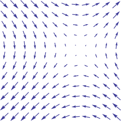
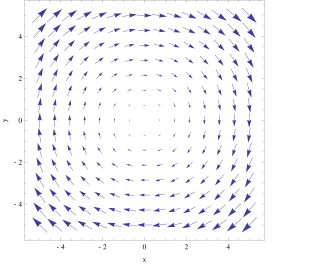
In vector calculus and physics, a vector field is an assignment of a vector to each point in a space, most commonly Euclidean space . A vector field on a plane can be visualized as a collection of arrows with given magnitudes and directions, each attached to a point on the plane. Vector fields are often used to model, for example, the speed and direction of a moving fluid throughout three dimensional space, such as the wind, or the strength and direction of some force, such as the magnetic or gravitational force, as it changes from one point to another point.
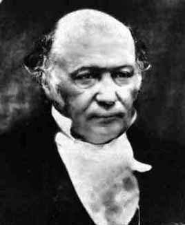
In physics, Hamiltonian mechanics is a reformulation of Lagrangian mechanics that emerged in 1833. Introduced by Sir William Rowan Hamilton, Hamiltonian mechanics replaces (generalized) velocities used in Lagrangian mechanics with (generalized) momenta. Both theories provide interpretations of classical mechanics and describe the same physical phenomena.
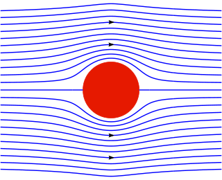
In fluid dynamics, two types of stream function are defined:

In special relativity, a four-vector is an object with four components, which transform in a specific way under Lorentz transformations. Specifically, a four-vector is an element of a four-dimensional vector space considered as a representation space of the standard representation of the Lorentz group, the representation. It differs from a Euclidean vector in how its magnitude is determined. The transformations that preserve this magnitude are the Lorentz transformations, which include spatial rotations and boosts.
In theoretical physics and mathematical physics, analytical mechanics, or theoretical mechanics is a collection of closely related formulations of classical mechanics. Analytical mechanics uses scalar properties of motion representing the system as a whole—usually its kinetic energy and potential energy. The equations of motion are derived from the scalar quantity by some underlying principle about the scalar's variation.

In mathematical physics, scalar potential describes the situation where the difference in the potential energies of an object in two different positions depends only on the positions, not upon the path taken by the object in traveling from one position to the other. It is a scalar field in three-space: a directionless value (scalar) that depends only on its location. A familiar example is potential energy due to gravity.
In the physical science of dynamics, rigid-body dynamics studies the movement of systems of interconnected bodies under the action of external forces. The assumption that the bodies are rigid simplifies analysis, by reducing the parameters that describe the configuration of the system to the translation and rotation of reference frames attached to each body. This excludes bodies that display fluid, highly elastic, and plastic behavior.
In continuum mechanics, the material derivative describes the time rate of change of some physical quantity of a material element that is subjected to a space-and-time-dependent macroscopic velocity field. The material derivative can serve as a link between Eulerian and Lagrangian descriptions of continuum deformation.
In mathematical analysis, and applications in geometry, applied mathematics, engineering, and natural sciences, a function of a real variable is a function whose domain is the real numbers , or a subset of that contains an interval of positive length. Most real functions that are considered and studied are differentiable in some interval. The most widely considered such functions are the real functions, which are the real-valued functions of a real variable, that is, the functions of a real variable whose codomain is the set of real numbers.

In geometry, a position or position vector, also known as location vector or radius vector, is a Euclidean vector that represents a point P in space. Its length represents the distance in relation to an arbitrary reference origin O, and its direction represents the angular orientation with respect to given reference axes. Usually denoted x, r, or s, it corresponds to the straight line segment from O to P. In other words, it is the displacement or translation that maps the origin to P:

In geometry, a three-dimensional space is a mathematical space in which three values (coordinates) are required to determine the position of a point. Most commonly, it is the three-dimensional Euclidean space, that is, the Euclidean space of dimension three, which models physical space. More general three-dimensional spaces are called 3-manifolds. The term may also refer colloquially to a subset of space, a three-dimensional region, a solid figure.
The gradient theorem, also known as the fundamental theorem of calculus for line integrals, says that a line integral through a gradient field can be evaluated by evaluating the original scalar field at the endpoints of the curve. The theorem is a generalization of the second fundamental theorem of calculus to any curve in a plane or space rather than just the real line.
In differential calculus, there is no single uniform notation for differentiation. Instead, various notations for the derivative of a function or variable have been proposed by various mathematicians. The usefulness of each notation varies with the context, and it is sometimes advantageous to use more than one notation in a given context. The most common notations for differentiation are listed below.

In physics, Lagrangian mechanics is a formulation of classical mechanics founded on the stationary-action principle. It was introduced by the Italian-French mathematician and astronomer Joseph-Louis Lagrange in his presentation to the Turin Academy of Science in 1760 culminating in his 1788 grand opus, Mécanique analytique.
In analytical mechanics and quantum field theory, minimal coupling refers to a coupling between fields which involves only the charge distribution and not higher multipole moments of the charge distribution. This minimal coupling is in contrast to, for example, Pauli coupling, which includes the magnetic moment of an electron directly in the Lagrangian.