Streamlines, streaklines, and pathlines

The red particle moves in a flowing fluid; its pathline is traced in red; the tip of the trail of blue ink released from the origin follows the particle, but unlike the static pathline (which records the earlier motion of the dot), ink released after the red dot departs continues to move up with the flow. (This is a streakline.) The dashed lines represent contours of the velocity field (streamlines), showing the motion of the whole field at the same time. (See high resolution version.)

Solid blue lines and broken grey lines represent the streamlines. The red arrows show the direction and magnitude of the flow velocity. These arrows are tangential to the streamline. The group of streamlines enclose the green curves (${\displaystyle C_{1}}$ and ${\displaystyle C_{2}}$) to form a stream surface.

Streamlines, streaklines and pathlines are field lines in a fluid flow. They differ only when the flow changes with time, that is, when the flow is not steady. ^{[1] [2]} Considering a velocity vector field in three-dimensional space in the framework of continuum mechanics, we have that:

• Streamlines are a family of curves whose tangent vectors constitute the velocity vector field of the flow. These show the direction in which a massless fluid element will travel at any point in time. ^[3]
• Streaklines are the loci of points of all the fluid particles that have passed continuously through a particular spatial point in the past. Dye steadily injected into the fluid at a fixed point (as in dye tracing) extends along a streakline.
• Pathlines are the trajectories that individual fluid particles follow. These can be thought of as "recording" the path of a fluid element in the flow over a certain period. The direction the path takes will be determined by the streamlines of the fluid at each moment in time.
• Timelines are the lines formed by a set of fluid particles that were marked at a previous instant in time, creating a line or a curve that is displaced in time as the particles move.

By definition, different streamlines at the same instant in a flow do not intersect, because a fluid particle cannot have two different velocities at the same point. However, pathlines are allowed to intersect themselves or other pathlines (except the starting and end points of the different pathlines, which need to be distinct). Streaklines can also intersect themselves and other streaklines.

Streamlines and timelines provide a snapshot of some flowfield characteristics, whereas streaklines and pathlines depend on the full time-history of the flow. However, often sequences of timelines (and streaklines) at different instants—being presented either in a single image or with a video stream—may be used to provide insight in the flow and its history.

If a line, curve or closed curve is used as start point for a continuous set of streamlines, the result is a stream surface. In the case of a closed curve in a steady flow, fluid that is inside a stream surface must remain forever within that same stream surface, because the streamlines are tangent to the flow velocity. A scalar function whose contour lines define the streamlines is known as the stream function .

Dye line may refer either to a streakline: dye released gradually from a fixed location during time; or it may refer to a timeline: a line of dye applied instantaneously at a certain moment in time, and observed at a later instant.

Mathematical description

Streamlines

The direction of magnetic field lines are streamlines represented by the alignment of iron filings sprinkled on paper placed above a bar magnet

Potential-flow streamlines achieving the Kutta condition around a NACA airfoil with upper and lower streamtubes identified.

Streamlines are defined by ^[4]

$${\displaystyle {d{\vec {x}}_{S} \over ds}\times {\vec {u}}({\vec {x}}_{S})={\vec {0}},}$$

where "${\displaystyle \times }$" denotes the vector cross product and ${\displaystyle {\vec {x}}_{S}(s)}$ is the parametric representation of just one streamline at one moment in time.

If the components of the velocity are written ${\displaystyle {\vec {u}}=(u,v,w),}$ and those of the streamline as ${\displaystyle {\vec {x}}_{S}=(x_{S},y_{S},z_{S}),}$ we deduce ^[4]

$${\displaystyle {dx_{S} \over u}={dy_{S} \over v}={dz_{S} \over w},}$$

which shows that the curves are parallel to the velocity vector. Here ${\displaystyle s}$ is a variable which parametrizes the curve ${\displaystyle s\mapsto {\vec {x}}_{S}(s).}$ Streamlines are calculated instantaneously, meaning that at one instance of time they are calculated throughout the fluid from the instantaneous flow velocity field.

A streamtube consists of a bundle of streamlines, much like communication cable.

The equation of motion of a fluid on a streamline for a flow in a vertical plane is: ^[5]

$${\displaystyle {\frac {\partial c}{\partial t}}+c{\frac {\partial c}{\partial s}}=\nu {\frac {\partial ^{2}c}{\partial r^{2}}}-{\frac {1}{\rho }}{\frac {\partial p}{\partial s}}-g{\frac {\partial z}{\partial s}}}$$

The flow velocity in the direction ${\displaystyle s}$ of the streamline is denoted by ${\displaystyle c}$. ${\displaystyle r}$ is the radius of curvature of the streamline. The density of the fluid is denoted by ${\displaystyle \rho }$ and the kinematic viscosity by ${\displaystyle \nu }$. ${\displaystyle {\frac {\partial p}{\partial s}}}$ is the pressure gradient and ${\displaystyle {\frac {\partial c}{\partial s}}}$ the velocity gradient along the streamline. For a steady flow, the time derivative of the velocity is zero: ${\displaystyle {\frac {\partial c}{\partial t}}=0}$. ${\displaystyle g}$ denotes the gravitational acceleration.

Pathlines

A long-exposure photo of spark from a campfire shows the pathlines for the flow of hot air.

Pathlines are defined by

$${\displaystyle {\begin{cases}{\dfrac {d{\vec {x}}_{P}}{dt}}(t)={\vec {u}}_{P}({\vec {x}}_{P}(t),t)\\[1.2ex]{\vec {x}}_{P}(t_{0})={\vec {x}}_{P0}\end{cases}}}$$

The subscript ${\displaystyle P}$ indicates that we are following the motion of a fluid particle. Note that at point ${\displaystyle {\vec {x}}_{P}}$ the curve is parallel to the flow velocity vector ${\displaystyle {\vec {u}}}$, where the velocity vector is evaluated at the position of the particle ${\displaystyle {\vec {x}}_{P}}$ at that time ${\displaystyle t}$.

Streaklines

Example of a streakline used to visualize the flow around a car inside a wind tunnel.

Streaklines can be expressed as,

$${\displaystyle {\begin{cases}\displaystyle {\frac {d{\vec {x}}_{str}}{dt}}={\vec {u}}_{P}({\vec {x}}_{str},t)\\[1.2ex]{\vec {x}}_{str}(t=\tau _{P})={\vec {x}}_{P0}\end{cases}}}$$

where, ${\displaystyle {\vec {u}}_{P}({\vec {x}},t)}$ is the velocity of a particle ${\displaystyle P}$ at location ${\displaystyle {\vec {x}}}$ and time ${\displaystyle t}$. The parameter ${\displaystyle \tau _{P}}$, parametrizes the streakline ${\displaystyle {\vec {x}}_{str}(t,\tau _{P})}$ and ${\displaystyle t_{0}\leq \tau _{P}\leq t}$, where ${\displaystyle t}$ is a time of interest.

Steady flows

In steady flow (when the velocity vector-field does not change with time), the streamlines, pathlines, and streaklines coincide. This is because when a particle on a streamline reaches a point, ${\displaystyle a_{0}}$, further on that streamline the equations governing the flow will send it in a certain direction ${\displaystyle {\vec {x}}}$. As the equations that govern the flow remain the same when another particle reaches ${\displaystyle a_{0}}$ it will also go in the direction ${\displaystyle {\vec {x}}}$. If the flow is not steady then when the next particle reaches position ${\displaystyle a_{0}}$ the flow would have changed and the particle will go in a different direction.

This is useful, because it is usually very difficult to look at streamlines in an experiment. However, if the flow is steady, one can use streaklines to describe the streamline pattern.

Frame dependence

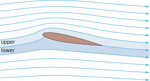
Streamlines are frame-dependent. That is, the streamlines observed in one inertial reference frame are different from those observed in another inertial reference frame. For instance, the streamlines in the air around an aircraft wing are defined differently for the passengers in the aircraft than for an observer on the ground. In the aircraft example, the observer on the ground will observe unsteady flow, and the observers in the aircraft will observe steady flow, with constant streamlines. When possible, fluid dynamicists try to find a reference frame in which the flow is steady, so that they can use experimental methods of creating streaklines to identify the streamlines.

Application

Knowledge of the streamlines can be useful in fluid dynamics. The curvature of a streamline is related to the pressure gradient acting perpendicular to the streamline. The center of curvature of the streamline lies in the direction of decreasing radial pressure. The magnitude of the radial pressure gradient can be calculated directly from the density of the fluid, the curvature of the streamline and the local velocity.

Dye can be used in water, or smoke in air, in order to see streaklines, from which pathlines can be calculated. Streaklines are identical to streamlines for steady flow. Further, dye can be used to create timelines. ^[6] The patterns guide design modifications, aiming to reduce the drag. This task is known as streamlining, and the resulting design is referred to as being streamlined. Streamlined objects and organisms, like airfoils, streamliners, cars and dolphins are often aesthetically pleasing to the eye. The Streamline Moderne style, a 1930s and 1940s offshoot of Art Deco, brought flowing lines to architecture and design of the era. The canonical example of a streamlined shape is a chicken egg with the blunt end facing forwards. This shows clearly that the curvature of the front surface can be much steeper than the back of the object. Most drag is caused by eddies in the fluid behind the moving object, and the objective should be to allow the fluid to slow down after passing around the object, and regain pressure, without forming eddies.

The same terms have since become common vernacular to describe any process that smooths an operation. For instance, it is common to hear references to streamlining a business practice, or operation.^{[ citation needed ]}

See also

• Physics portal

• Drag coefficient
• Elementary flow
• Equipotential surface
• Flow visualization
• Flow velocity
• Scientific visualization
• Seeding (fluid dynamics)
• Stream function
• Streamsurface
• Streamlet (scientific visualization)

Notes and references

Notes

1. Batchelor, G. (2000). Introduction to Fluid Mechanics.
2. Kundu P and Cohen I. Fluid Mechanics.
3. "Definition of Streamlines". www.grc.nasa.gov. Archived from the original on 18 January 2017. Retrieved 4 October 2023.
4. Granger, R.A. (1995). Fluid Mechanics. Dover Publications. ISBN   0-486-68356-7., pp. 422–425.
5. tec-science (2020-04-22). "Equation of motion of a fluid on a streamline". tec-science. Retrieved 2020-05-07.
6. "Flow visualisation". National Committee for Fluid Mechanics Films (NCFMF). Archived from the original (RealMedia) on 2006-01-03. Retrieved 2009-04-20.

References

• Faber, T.E. (1995). Fluid Dynamics for Physicists. Cambridge University Press. ISBN   0-521-42969-2.

External links

• Streamline illustration
• Tutorial - Illustration of Streamlines, Streaklines and Pathlines of a Velocity Field(with applet)
• Joukowsky Transform Interactive WebApp