Tangent

For the tangent function, see Tangent (trigonometry). For other uses, see Tangent (disambiguation).

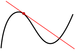
Tangent to a curve. The red line is tangential to the curve at the point marked by a red dot.

Tangent plane to a sphere

In geometry, the tangent line (or simply tangent) to a plane curve at a given point is, intuitively, the straight line that "just touches" the curve at that point. Leibniz defined it as the line through a pair of infinitely close points on the curve. ^{[1] [2]} More precisely, a straight line is tangent to the curve y = f(x) at a point x = c if the line passes through the point (c, f(c)) on the curve and has slope f'(c), where f' is the derivative of f. A similar definition applies to space curves and curves in n-dimensional Euclidean space.

The point where the tangent line and the curve meet or intersect is called the point of tangency. The tangent line is said to be "going in the same direction" as the curve, and is thus the best straight-line approximation to the curve at that point. The tangent line to a point on a differentiable curve can also be thought of as a tangent line approximation , the graph of the affine function that best approximates the original function at the given point. ^[3]

Similarly, the tangent plane to a surface at a given point is the plane that "just touches" the surface at that point. The concept of a tangent is one of the most fundamental notions in differential geometry and has been extensively generalized; see Tangent space .

The word "tangent" comes from the Latin tangere , "to touch".

History

Euclid makes several references to the tangent (ἐφαπτομένηephaptoménē) to a circle in book III of the Elements (c. 300 BC). ^[4] In Apollonius' work Conics (c. 225 BC) he defines a tangent as being a line such that no other straight line could fall between it and the curve. ^[5]

Archimedes (c.  287 – c.  212 BC) found the tangent to an Archimedean spiral by considering the path of a point moving along the curve. ^[5]

In the 1630s Fermat developed the technique of adequality to calculate tangents and other problems in analysis and used this to calculate tangents to the parabola. The technique of adequality is similar to taking the difference between ${\displaystyle f(x+h)}$ and ${\displaystyle f(x)}$ and dividing by a power of ${\displaystyle h}$. Independently Descartes used his method of normals based on the observation that the radius of a circle is always normal to the circle itself. ^[6]

These methods led to the development of differential calculus in the 17th century. Many people contributed. Roberval discovered a general method of drawing tangents, by considering a curve as described by a moving point whose motion is the resultant of several simpler motions. ^[7] René-François de Sluse and Johannes Hudde found algebraic algorithms for finding tangents. ^[8] Further developments included those of John Wallis and Isaac Barrow, leading to the theory of Isaac Newton and Gottfried Leibniz.

An 1828 definition of a tangent was "a right line which touches a curve, but which when produced, does not cut it". ^[9] This old definition prevents inflection points from having any tangent. It has been dismissed and the modern definitions are equivalent to those of Leibniz, who defined the tangent line as the line through a pair of infinitely close points on the curve.

Tangent line to a plane curve

Further information: Differentiable curve § Tangent vector, and Frenet–Serret formulas

A tangent, a chord, and a secant to a circle

The intuitive notion that a tangent line "touches" a curve can be made more explicit by considering the sequence of straight lines (secant lines) passing through two points, A and B, those that lie on the function curve. The tangent at A is the limit when point B approximates or tends to A. The existence and uniqueness of the tangent line depends on a certain type of mathematical smoothness, known as "differentiability." For example, if two circular arcs meet at a sharp point (a vertex) then there is no uniquely defined tangent at the vertex because the limit of the progression of secant lines depends on the direction in which "point B" approaches the vertex.

At most points, the tangent touches the curve without crossing it (though it may, when continued, cross the curve at other places away from the point of tangent). A point where the tangent (at this point) crosses the curve is called an inflection point . Circles, parabolas, hyperbolas and ellipses do not have any inflection point, but more complicated curves do have, like the graph of a cubic function, which has exactly one inflection point, or a sinusoid, which has two inflection points per each period of the sine.

Conversely, it may happen that the curve lies entirely on one side of a straight line passing through a point on it, and yet this straight line is not a tangent line. This is the case, for example, for a line passing through the vertex of a triangle and not intersecting it otherwise—where the tangent line does not exist for the reasons explained above. In convex geometry, such lines are called supporting lines.

Analytical approach

At each point, the moving line is always tangent to the curve. Its slope is the derivative; green marks positive derivative, red marks negative derivative and black marks zero derivative. The point (x,y) = (0,1) where the tangent intersects the curve, is not a max, or a min, but is a point of inflection. (Note: the figure contains the incorrect labeling of 0,0 which should be 0,1)

The geometrical idea of the tangent line as the limit of secant lines serves as the motivation for analytical methods that are used to find tangent lines explicitly. The question of finding the tangent line to a graph, or the tangent line problem, was one of the central questions leading to the development of calculus in the 17th century. In the second book of his Geometry , René Descartes ^[10] said of the problem of constructing the tangent to a curve, "And I dare say that this is not only the most useful and most general problem in geometry that I know, but even that I have ever desired to know". ^[11]

Intuitive description

Suppose that a curve is given as the graph of a function, y = f(x). To find the tangent line at the point p = (a, f(a)), consider another nearby point q = (a + h, f(a + h)) on the curve. The slope of the secant line passing through p and q is equal to the difference quotient

${\displaystyle {\frac {f(a+h)-f(a)}{h}}.}$

As the point q approaches p, which corresponds to making h smaller and smaller, the difference quotient should approach a certain limiting value k, which is the slope of the tangent line at the point p. If k is known, the equation of the tangent line can be found in the point-slope form:

${\displaystyle y-f(a)=k(x-a).\,}$

More rigorous description

To make the preceding reasoning rigorous, one has to explain what is meant by the difference quotient approaching a certain limiting value k. The precise mathematical formulation was given by Cauchy in the 19th century and is based on the notion of limit. Suppose that the graph does not have a break or a sharp edge at p and it is neither plumb nor too wiggly near p. Then there is a unique value of k such that, as h approaches 0, the difference quotient gets closer and closer to k, and the distance between them becomes negligible compared with the size of h, if h is small enough. This leads to the definition of the slope of the tangent line to the graph as the limit of the difference quotients for the function f. This limit is the derivative of the function f at x = a, denoted f ′(a). Using derivatives, the equation of the tangent line can be stated as follows:

${\displaystyle y=f(a)+f'(a)(x-a).\,}$

Calculus provides rules for computing the derivatives of functions that are given by formulas, such as the power function, trigonometric functions, exponential function, logarithm, and their various combinations. Thus, equations of the tangents to graphs of all these functions, as well as many others, can be found by the methods of calculus.

How the method can fail

Calculus also demonstrates that there are functions and points on their graphs for which the limit determining the slope of the tangent line does not exist. For these points the function f is non-differentiable. There are two possible reasons for the method of finding the tangents based on the limits and derivatives to fail: either the geometric tangent exists, but it is a vertical line, which cannot be given in the point-slope form since it does not have a slope, or the graph exhibits one of three behaviors that precludes a geometric tangent.

The graph y = x^1/3 illustrates the first possibility: here the difference quotient at a = 0 is equal to h^1/3/h = h^−2/3, which becomes very large as h approaches 0. This curve has a tangent line at the origin that is vertical.

The graph y = x^2/3 illustrates another possibility: this graph has a cusp at the origin. This means that, when h approaches 0, the difference quotient at a = 0 approaches plus or minus infinity depending on the sign of x. Thus both branches of the curve are near to the half vertical line for which y=0, but none is near to the negative part of this line. Basically, there is no tangent at the origin in this case, but in some context one may consider this line as a tangent, and even, in algebraic geometry, as a double tangent.

The graph y = |x| of the absolute value function consists of two straight lines with different slopes joined at the origin. As a point q approaches the origin from the right, the secant line always has slope 1. As a point q approaches the origin from the left, the secant line always has slope −1. Therefore, there is no unique tangent to the graph at the origin. Having two different (but finite) slopes is called a corner.

Finally, since differentiability implies continuity, the contrapositive states discontinuity implies non-differentiability. Any such jump or point discontinuity will have no tangent line. This includes cases where one slope approaches positive infinity while the other approaches negative infinity, leading to an infinite jump discontinuity

Equations

When the curve is given by y = f(x) then the slope of the tangent is ${\displaystyle dy/dx,}$ so by the point–slope formula the equation of the tangent line at (X, Y) is

${\displaystyle y-Y={\frac {dy}{dx}}(X)\cdot (x-X)}$

where (x, y) are the coordinates of any point on the tangent line, and where the derivative is evaluated at ${\displaystyle x=X}$. ^[12]

When the curve is given by y = f(x), the tangent line's equation can also be found ^[13] by using polynomial division to divide ${\displaystyle f\,(x)}$ by ${\displaystyle (x-X)^{2}}$; if the remainder is denoted by ${\displaystyle g(x)}$, then the equation of the tangent line is given by

${\displaystyle y=g(x).}$

When the equation of the curve is given in the form f(x, y) = 0 then the value of the slope can be found by implicit differentiation, giving

${\displaystyle {\frac {dy}{dx}}=-{\frac {\partial f}{\partial x}}{\bigg /}{\frac {\partial f}{\partial y}}.}$

The equation of the tangent line at a point (X,Y) such that f(X,Y) = 0 is then ^[12]

${\displaystyle {\frac {\partial f}{\partial x}}(X,Y)\cdot (x-X)+{\frac {\partial f}{\partial y}}(X,Y)\cdot (y-Y)=0.}$

This equation remains true if

${\displaystyle {\frac {\partial f}{\partial y}}(X,Y)=0,\quad {\frac {\partial f}{\partial x}}(X,Y)\neq 0,}$

in which case the slope of the tangent is infinite. If, however,

${\displaystyle {\frac {\partial f}{\partial y}}(X,Y)={\frac {\partial f}{\partial x}}(X,Y)=0,}$

the tangent line is not defined and the point (X,Y) is said to be singular.

For algebraic curves, computations may be simplified somewhat by converting to homogeneous coordinates. Specifically, let the homogeneous equation of the curve be g(x, y, z) = 0 where g is a homogeneous function of degree n. Then, if (X, Y, Z) lies on the curve, Euler's theorem implies

$${\displaystyle {\frac {\partial g}{\partial x}}\cdot X+{\frac {\partial g}{\partial y}}\cdot Y+{\frac {\partial g}{\partial z}}\cdot Z=ng(X,Y,Z)=0.}$$

It follows that the homogeneous equation of the tangent line is

${\displaystyle {\frac {\partial g}{\partial x}}(X,Y,Z)\cdot x+{\frac {\partial g}{\partial y}}(X,Y,Z)\cdot y+{\frac {\partial g}{\partial z}}(X,Y,Z)\cdot z=0.}$

The equation of the tangent line in Cartesian coordinates can be found by setting z=1 in this equation. ^[14]

To apply this to algebraic curves, write f(x, y) as

${\displaystyle f=u_{n}+u_{n-1}+\dots +u_{1}+u_{0}\,}$

where each u_r is the sum of all terms of degree r. The homogeneous equation of the curve is then

${\displaystyle g=u_{n}+u_{n-1}z+\dots +u_{1}z^{n-1}+u_{0}z^{n}=0.\,}$

Applying the equation above and setting z=1 produces

${\displaystyle {\frac {\partial f}{\partial x}}(X,Y)\cdot x+{\frac {\partial f}{\partial y}}(X,Y)\cdot y+{\frac {\partial g}{\partial z}}(X,Y,1)=0}$

as the equation of the tangent line. ^[15] The equation in this form is often simpler to use in practice since no further simplification is needed after it is applied. ^[14]

If the curve is given parametrically by

${\displaystyle x=x(t),\quad y=y(t)}$

then the slope of the tangent is

${\displaystyle {\frac {dy}{dx}}={\frac {dy}{dt}}{\bigg /}{\frac {dx}{dt}}}$

giving the equation for the tangent line at ${\displaystyle \,t=T,\,X=x(T),\,Y=y(T)}$ as ^[16]

${\displaystyle {\frac {dx}{dt}}(T)\cdot (y-Y)={\frac {dy}{dt}}(T)\cdot (x-X).}$

If

${\displaystyle {\frac {dx}{dt}}(T)={\frac {dy}{dt}}(T)=0,}$

the tangent line is not defined. However, it may occur that the tangent line exists and may be computed from an implicit equation of the curve.

Normal line to a curve

Further information: Normal (geometry)

The line perpendicular to the tangent line to a curve at the point of tangency is called the normal line to the curve at that point. The slopes of perpendicular lines have product −1, so if the equation of the curve is y = f(x) then slope of the normal line is

${\displaystyle -1{\bigg /}{\frac {dy}{dx}}}$

and it follows that the equation of the normal line at (X, Y) is

${\displaystyle (x-X)+{\frac {dy}{dx}}(y-Y)=0.}$

Similarly, if the equation of the curve has the form f(x, y) = 0 then the equation of the normal line is given by ^[17]

${\displaystyle {\frac {\partial f}{\partial y}}(x-X)-{\frac {\partial f}{\partial x}}(y-Y)=0.}$

If the curve is given parametrically by

${\displaystyle x=x(t),\quad y=y(t)}$

then the equation of the normal line is ^[16]

${\displaystyle {\frac {dx}{dt}}(x-X)+{\frac {dy}{dt}}(y-Y)=0.}$

Angle between curves

See also: Angle § Angles between curves

The angle between two curves at a point where they intersect is defined as the angle between their tangent lines at that point. More specifically, two curves are said to be tangent at a point if they have the same tangent at a point, and orthogonal if their tangent lines are orthogonal. ^[18]

Multiple tangents at a point

The limaçon trisectrix: a curve with two tangents at the origin.

The formulas above fail when the point is a singular point. In this case there may be two or more branches of the curve that pass through the point, each branch having its own tangent line. When the point is the origin, the equations of these lines can be found for algebraic curves by factoring the equation formed by eliminating all but the lowest degree terms from the original equation. Since any point can be made the origin by a change of variables (or by translating the curve) this gives a method for finding the tangent lines at any singular point.

For example, the equation of the limaçon trisectrix shown to the right is

${\displaystyle (x^{2}+y^{2}-2ax)^{2}=a^{2}(x^{2}+y^{2}).\,}$

Expanding this and eliminating all but terms of degree 2 gives

${\displaystyle a^{2}(3x^{2}-y^{2})=0\,}$

which, when factored, becomes

${\displaystyle y=\pm {\sqrt {3}}x.}$

So these are the equations of the two tangent lines through the origin. ^[19]

When the curve is not self-crossing, the tangent at a reference point may still not be uniquely defined because the curve is not differentiable at that point although it is differentiable elsewhere. In this case the left and right derivatives are defined as the limits of the derivative as the point at which it is evaluated approaches the reference point from respectively the left (lower values) or the right (higher values). For example, the curve y = |x | is not differentiable at x = 0: its left and right derivatives have respective slopes −1 and 1; the tangents at that point with those slopes are called the left and right tangents. ^[20]

Sometimes the slopes of the left and right tangent lines are equal, so the tangent lines coincide. This is true, for example, for the curve y = x^2/3, for which both the left and right derivatives at x = 0 are infinite; both the left and right tangent lines have equation x = 0.

Tangent line to a space curve

This section is an excerpt from Tangent vector.[ edit ]

In mathematics, a tangent vector is a vector that is tangent to a curve or surface at a given point. Tangent vectors are described in the differential geometry of curves in the context of curves in Rⁿ. More generally, tangent vectors are elements of a tangent space of a differentiable manifold. Tangent vectors can also be described in terms of germs. Formally, a tangent vector at the point ${\displaystyle x}$ is a linear derivation of the algebra defined by the set of germs at ${\displaystyle x}$.

Tangent circles

Main article: Tangent circles

Two pairs of tangent circles. Above internally and below externally tangent

Two distinct circles lying in the same plane are said to be tangent to each other if they meet at exactly one point.

If points in the plane are described using Cartesian coordinates, then two circles, with radii ${\displaystyle r_{1},r_{2}}$ and centers ${\displaystyle (x_{1},y_{1})}$ and ${\displaystyle (x_{2},y_{2})}$ are tangent to each other whenever

${\displaystyle \left(x_{1}-x_{2}\right)^{2}+\left(y_{1}-y_{2}\right)^{2}=\left(r_{1}\pm r_{2}\right)^{2}.}$

The two circles are called externally tangent if the distance between their centres is equal to the sum of their radii,

${\displaystyle \left(x_{1}-x_{2}\right)^{2}+\left(y_{1}-y_{2}\right)^{2}=\left(r_{1}+r_{2}\right)^{2}.}$

or internally tangent if the distance between their centres is equal to the difference between their radii: ^[21]

${\displaystyle \left(x_{1}-x_{2}\right)^{2}+\left(y_{1}-y_{2}\right)^{2}=\left(r_{1}-r_{2}\right)^{2}.}$

Tangent plane to a surface

"Tangent plane" redirects here. For the geographical concept, see Local tangent plane.

Further information: Differential geometry of surfaces § Tangent plane, and Parametric surface § Tangent plane

See also: Normal plane (geometry)

The tangent plane to a surface at a given point p is defined in an analogous way to the tangent line in the case of curves. It is the best approximation of the surface by a plane at p, and can be obtained as the limiting position of the planes passing through 3 distinct points on the surface close to p as these points converge to p. Mathematically, if the surface is given by a function ${\displaystyle z=f(x,y)}$, the equation of the tangent plane at point ${\displaystyle (x_{0},y_{0},z_{0})}$ can be expressed as:

${\displaystyle z-z_{0}={\frac {\partial f}{\partial x}}(x_{0},y_{0})(x-x_{0})+{\frac {\partial f}{\partial y}}(x_{0},y_{0})(y-y_{0})}$.

Here, ${\textstyle {\frac {\partial f}{\partial x}}}$ and ${\textstyle {\frac {\partial f}{\partial y}}}$ are the partial derivatives of the function ${\displaystyle f}$ with respect to ${\displaystyle x}$ and ${\displaystyle y}$ respectively, evaluated at the point ${\displaystyle (x_{0},y_{0})}$. In essence, the tangent plane captures the local behavior of the surface at the specific point p. It's a fundamental concept used in calculus and differential geometry, crucial for understanding how functions change locally on surfaces.

Higher-dimensional manifolds

Main article: Tangent space

More generally, there is a k-dimensional tangent space at each point of a k-dimensional manifold in the n-dimensional Euclidean space.

See also

• Newton's method
• Normal (geometry)
• Osculating circle
• Osculating curve
• Perpendicular
• Subtangent
• Supporting line
• Tangent cone
• Tangential angle
• Tangential component
• Tangent lines to circles
• Tangent vector
• Multiplicity (mathematics)#Behavior of a polynomial function near a multiple root
• Algebraic curve#Tangent at a point

References

1. In "Nova Methodus pro Maximis et Minimis" ( Acta Eruditorum , Oct. 1684), Leibniz appears to have a notion of tangent lines readily from the start, but later states: "modo teneatur in genere, tangentem invenire esse rectam ducere, quae duo curvae puncta distantiam infinite parvam habentia jungat, seu latus productum polygoni infinitanguli, quod nobis curvae aequivalet", ie. defines the method for drawing tangents through points infinitely close to each other.
2. Thomas L. Hankins (1985). Science and the Enlightenment. Cambridge University Press. p. 23. ISBN   9780521286190.
3. Dan Sloughter (2000) . "Best Affine Approximations"
4. Euclid. "Euclid's Elements" . Retrieved 1 June 2015.
5. Shenk, Al. "e-CALCULUS Section 2.8" (PDF). p. 2.8. Retrieved 1 June 2015.
6. Katz, Victor J. (2008). A History of Mathematics (3rd ed.). Addison Wesley. p. 510. ISBN   978-0321387004.
7. Wolfson, Paul R. (2001). "The Crooked Made Straight: Roberval and Newton on Tangents". The American Mathematical Monthly. 108 (3): 206–216. doi:10.2307/2695381. JSTOR   2695381.
8. Katz, Victor J. (2008). A History of Mathematics (3rd ed.). Addison Wesley. pp. 512–514. ISBN   978-0321387004.
9. Noah Webster, American Dictionary of the English Language (New York: S. Converse, 1828), vol. 2, p. 733,
10. Descartes, René (1954) [1637]. The Geometry of René Descartes. Translated by Smith, David Eugene; Latham, Marcia L. Open Court. p. 95.
11. R. E. Langer (October 1937). "Rene Descartes". American Mathematical Monthly . Mathematical Association of America. 44 (8): 495–512. doi:10.2307/2301226. JSTOR   2301226.
12. Edwards Art. 191
13. Strickland-Constable, Charles, "A simple method for finding tangents to polynomial graphs", Mathematical Gazette , November 2005, 466–467.
14. Edwards Art. 192
15. Edwards Art. 193
16. Edwards Art. 196
17. Edwards Art. 194
18. Edwards Art. 195
19. Edwards Art. 197
20. Thomas, George B. Jr., and Finney, Ross L. (1979), Calculus and Analytic Geometry, Addison Wesley Publ. Co.: p. 140.
21. "Circles For Leaving Certificate Honours Mathematics by Thomas O'Sullivan 1997".

Sources

• J. Edwards (1892). Differential Calculus. London: MacMillan and Co. pp.  143 ff.

External links

• "Tangent line", Encyclopedia of Mathematics , EMS Press, 2001 [1994]
• Weisstein, Eric W. "Tangent Line". MathWorld .
• Tangent to a circle With interactive animation
• Tangent and first derivative — An interactive simulation