Archimedean spiral

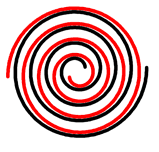
Three 360° loops of one arm of an Archimedean spiral

The Archimedean spiral (also known as the arithmetic spiral) is a spiral named after the 3rd-century BC Greek mathematician Archimedes. It is the locus corresponding to the locations over time of a point moving away from a fixed point with a constant speed along a line that rotates with constant angular velocity. Equivalently, in polar coordinates (r, θ) it can be described by the equation

$${\displaystyle r=b\cdot \theta }$$

with real number b. Changing the parameter b controls the distance between loops.

From the above equation, it can thus be stated: position of particle from point of start is proportional to angle θ as time elapses.

Archimedes described such a spiral in his book On Spirals . Conon of Samos was a friend of his and Pappus states that this spiral was discovered by Conon. ^[1]

Derivation of general equation of spiral

See also: Circular motion

A physical approach is used below to understand the notion of Archimedean spirals.

Suppose a point object moves in the Cartesian system with a constant velocity v directed parallel to the x-axis, with respect to the xy-plane. Let at time t = 0, the object was at an arbitrary point (c, 0, 0). If the xy plane rotates with a constant angular velocity ω about the z-axis, then the velocity of the point with respect to z-axis may be written as:

The xy plane rotates to an angle ωt (anticlockwise) about the origin in time t. (c, 0) is the position of the object at t = 0. P is the position of the object at time t, at a distance of R = vt + c.

$${\displaystyle {\begin{aligned}|v_{0}|&={\sqrt {v^{2}+\omega ^{2}(vt+c)^{2}}}\\v_{x}&=v\cos \omega t-\omega (vt+c)\sin \omega t\\v_{y}&=v\sin \omega t+\omega (vt+c)\cos \omega t\end{aligned}}}$$

As shown in the figure alongside, we have vt + c representing the modulus of the position vector of the particle at any time t, with v_x and v_y as the velocity components along the x and y axes, respectively.

$${\displaystyle {\begin{aligned}\int v_{x}\,dt&=x\\\int v_{y}\,dt&=y\end{aligned}}}$$

The above equations can be integrated by applying integration by parts, leading to the following parametric equations:

$${\displaystyle {\begin{aligned}x&=(vt+c)\cos \omega t\\y&=(vt+c)\sin \omega t\end{aligned}}}$$

Squaring the two equations and then adding (and some small alterations) results in the Cartesian equation

$${\displaystyle {\sqrt {x^{2}+y^{2}}}={\frac {v}{\omega }}\cdot \arctan {\frac {y}{x}}+c}$$

(using the fact that ωt = θ and θ = arctan y/x) or

$${\displaystyle \tan \left(\left({\sqrt {x^{2}+y^{2}}}-c\right)\cdot {\frac {\omega }{v}}\right)={\frac {y}{x}}}$$

Its polar form is

$${\displaystyle r={\frac {v}{\omega }}\cdot \theta +c.}$$

Arc length and curvature

Osculating circles of the Archimedean spiral, tangent to the spiral and having the same curvature at the tangent point. The spiral itself is not drawn, but can be seen as the points where the circles are especially close to each other.

Given the parametrization in cartesian coordinates

$${\displaystyle f\colon \theta \mapsto (r\,\cos \theta ,r\,\sin \theta )=(b\,\theta \,\cos \theta ,b\,\theta \,\sin \theta )}$$

the arc length from θ₁ to θ₂ is

$${\displaystyle {\frac {b}{2}}\left[\theta \,{\sqrt {1+\theta ^{2}}}+\ln \left(\theta +{\sqrt {1+\theta ^{2}}}\right)\right]_{\theta _{1}}^{\theta _{2}}}$$

or, equivalently:

$${\displaystyle {\frac {b}{2}}\left[\theta \,{\sqrt {1+\theta ^{2}}}+\operatorname {arsinh} \theta \right]_{\theta _{1}}^{\theta _{2}}.}$$

The total length from θ₁ = 0 to θ₂ = θ is therefore

$${\displaystyle {\frac {b}{2}}\left[\theta \,{\sqrt {1+\theta ^{2}}}+\ln \left(\theta +{\sqrt {1+\theta ^{2}}}\right)\right].}$$

The curvature is given by

$${\displaystyle \kappa ={\frac {\theta ^{2}+2}{b\left(\theta ^{2}+1\right)^{\frac {3}{2}}}}}$$

Characteristics

Archimedean spiral represented on a polar graph

The Archimedean spiral has the property that any ray from the origin intersects successive turnings of the spiral in points with a constant separation distance (equal to 2 πb if θ is measured in radians), hence the name "arithmetic spiral". In contrast to this, in a logarithmic spiral these distances, as well as the distances of the intersection points measured from the origin, form a geometric progression.

The Archimedean spiral has two arms, one for θ > 0 and one for θ < 0. The two arms are smoothly connected at the origin. Only one arm is shown on the accompanying graph. Taking the mirror image of this arm across the y-axis will yield the other arm.

For large θ a point moves with well-approximated uniform acceleration along the Archimedean spiral while the spiral corresponds to the locations over time of a point moving away from a fixed point with a constant speed along a line which rotates with constant angular velocity ^[2] (see contribution from Mikhail Gaichenkov).

As the Archimedean spiral grows, its evolute asymptotically approaches a circle with radius |v|/ω.

General Archimedean spiral

Sometimes the term Archimedean spiral is used for the more general group of spirals

$${\displaystyle r=a+b\cdot \theta ^{\frac {1}{c}}.}$$

The normal Archimedean spiral occurs when c = 1. Other spirals falling into this group include the hyperbolic spiral (c = −1), Fermat's spiral (c = 2), and the lituus (c = −2).

Applications

One method of squaring the circle, due to Archimedes, makes use of an Archimedean spiral. Archimedes also showed how the spiral can be used to trisect an angle. Both approaches relax the traditional limitations on the use of straightedge and compass in ancient Greek geometric proofs. ^[3]

Mechanism of a scroll compressor

The Archimedean spiral has a variety of real-world applications. Scroll compressors, used for compressing gases, have rotors that can be made from two interleaved Archimedean spirals, involutes of a circle of the same size that almost resemble Archimedean spirals, ^[4] or hybrid curves.

Archimedean spirals can be found in spiral antenna, which can be operated over a wide range of frequencies.

The coils of watch balance springs and the grooves of very early gramophone records form Archimedean spirals, making the grooves evenly spaced (although variable track spacing was later introduced to maximize the amount of music that could be cut onto a record). ^[5]

Asking for a patient to draw an Archimedean spiral is a way of quantifying human tremor; this information helps in diagnosing neurological diseases.

Archimedean spirals are also used in digital light processing (DLP) projection systems to minimize the "rainbow effect", making it look as if multiple colors are displayed at the same time, when in reality red, green, and blue are being cycled extremely quickly. ^[6] Additionally, Archimedean spirals are used in food microbiology to quantify bacterial concentration through a spiral platter. ^[7]

Atacama Large Millimeter Array image of LL Pegasi

They are also used to model the pattern that occurs in a roll of paper or tape of constant thickness wrapped around a cylinder. ^{[8] [9]}

Many dynamic spirals (such as the Parker spiral of the solar wind, or the pattern made by a Catherine's wheel) are Archimedean. For instance, the star LL Pegasi shows an approximate Archimedean spiral in the dust clouds surrounding it, thought to be ejected matter from the star that has been shepherded into a spiral by another companion star as part of a double star system. ^[10]

See also

• Mathematics portal

• Archimedes' screw  – Water pumping mechanism ^[11]
• Fermat's spiral  – Spiral that surrounds equal area per turn
• Golden spiral  – Self-similar curve related to golden ratio
• Hyperbolic spiral  – Spiral asymptotic to a line
• List of spirals
• Logarithmic spiral  – Self-similar growth curve
• Spiral of Theodorus  – Polygonal curve made from right triangles
• Triple spiral symbol  – Various symbols with three-fold rotational symmetryPages displaying short descriptions of redirect targets

References

1. Bulmer-Thomas, Ivor. "Conon of Samos". Dictionary of Scientific Biography . Vol. 3. p. 391.
2. Sloane, N. J. A. (ed.). "SequenceA091154". The On-Line Encyclopedia of Integer Sequences . OEIS Foundation.
3. Boyer, Carl B. (1968). A History of Mathematics. Princeton, New Jersey: Princeton University Press. pp. 140–142. ISBN   0-691-02391-3.
4. Sakata, Hirotsugu; Okuda, Masayuki. "Fluid compressing device having coaxial spiral members" . Retrieved 2006-11-25.
5. Penndorf, Ron. "Early Development of the LP". Archived from the original on 5 November 2005. Retrieved 2005-11-25.. See the passage on Variable Groove.
6. Ballou, Glen (2008), Handbook for Sound Engineers, CRC Press, p. 1586, ISBN   9780240809694
7. Gilchrist, J. E.; Campbell, J. E.; Donnelly, C. B.; Peeler, J. T.; Delaney, J. M. (1973). "Spiral Plate Method for Bacterial Determination". Applied Microbiology. 25 (2): 244–52. doi:10.1128/AEM.25.2.244-252.1973. PMC   380780 . PMID   4632851.
8. Peressini, Tony (3 February 2009). "Joan's Paper Roll Problem" (PDF). Archived from the original (PDF) on 3 November 2013. Retrieved 2014-10-06.
9. Walser, H.; Hilton, P.; Pedersen, J. (2000). Symmetry . Mathematical Association of America. p.  27. ISBN   9780883855324 . Retrieved 2014-10-06.
10. Kim, Hyosun; Trejo, Alfonso; Liu, Sheng-Yuan; Sahai, Raghvendra; Taam, Ronald E.; Morris, Mark R.; Hirano, Naomi; Hsieh, I-Ta (March 2017). "The large-scale nebular pattern of a superwind binary in an eccentric orbit". Nature Astronomy. 1 (3): 0060. arXiv: 1704.00449 . Bibcode:2017NatAs...1E..60K. doi:10.1038/s41550-017-0060. S2CID   119433782.

External links

• Jonathan Matt making the Archimedean spiral interesting - Video : The surprising beauty of Mathematics - TedX Talks, Green Farms
• Weisstein, Eric W. "Archimedes' Spiral". MathWorld .
• archimedean spiral at PlanetMath .
• Page with Java application to interactively explore the Archimedean spiral and its related curves
• Online exploration using JSXGraph (JavaScript)
• Archimedean spiral at "mathcurve"