This list of spirals includes named spirals that have been described mathematically.
| Image | Name | First described | Equation | Comment |
|---|---|---|---|---|
 | Circle | The trivial spiral | ||
 | Archimedean spiral (also arithmetic spiral) | c. 320 BC | ||
 | Fermat's spiral (also parabolic spiral) | 1636 [1] | Encloses equal area per turn | |
 | Doyle spiral | 1980—1990 [2] | circle packing, using circles of structured radii | |
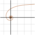
 | Euler spiral (also Cornu spiral or polynomial spiral) | 1696 [3] | Using Fresnel integrals [4] | |
 | Hyperbolic spiral (also reciprocal spiral) | 1704 | ||
 | Lituus | 1722 | ||
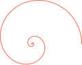
 | Logarithmic spiral (also known as equiangular spiral) | 1638 [5] | Constant pitch angle. Approximations of this are found in nature | |
 | Fibonacci spiral | Circular arcs connecting the opposite corners of squares in the Fibonacci tiling | Approximation of the golden spiral | |
 | Golden spiral | Special case of the logarithmic spiral | ||
 | Spiral of Theodorus (also known as Pythagorean spiral) | c. 500 BC | Contiguous right triangles composed of one leg with unit length and the other leg being the hypotenuse of the prior triangle | Approximates the Archimedean spiral |
 | Involute | 1673 | Involutes of a circle appear like Archimedean spirals | |
 | Helix | A three-dimensional spiral | ||
 | Rhumb line (also loxodrome) | Type of spiral drawn on a sphere | ||
 | Cotes's spiral | 1722 | Solution to the two-body problem for an inverse-cube central force | |
 | Poinsot's spirals | |||
 | Nielsen's spiral | 1993 [6] | A variation of Euler spiral, using sine integral and cosine integrals | |
 | Polygonal spiral | Special case approximation of arithmetic or logarithmic spiral | ||
 | Fraser's Spiral | 1908 | Optical illusion based on spirals | |
 | Conchospiral | A three-dimensional spiral on the surface of a cone. | ||
 | Calkin–Wilf spiral | |||
 | Ulam spiral (also prime spiral) | 1963 | ||
 | Sacks spiral | 1994 | Variant of Ulam spiral and Archimedean spiral. | |
| Seiffert's spiral | 2000 [7] | Spiral curve on the surface of a sphere using the Jacobi elliptic functions [8] | ||
 | Tractrix spiral | 1704 [9] | ||
| Pappus spiral | 1779 | 3D conical spiral studied by Pappus and Pascal [10] | ||
 | Doppler spiral | 2D projection of Pappus spiral [11] | ||
 | Atzema spiral | The curve that has a catacaustic forming a circle. Approximates the Archimedean spiral. [12] | ||
 | Atomic spiral | 2002 | This spiral has two asymptotes; one is the circle of radius 1 and the other is the line [13] | |
 | Galactic spiral | 2019 | The differential spiral equations were developed to simulate the spiral arms of disc galaxies, have 4 solutions with three different cases:, the spiral patterns are decided by the behavior of the parameter . For , spiral-ring pattern; regular spiral; loose spiral. R is the distance of spiral starting point (0, R) to the center. The calculated x and y have to be rotated backward by () for plotting. [14] [ predatory publisher ] |


