Polar coordinate system

Points in the polar coordinate system with pole O and polar axis L. In green, the point with radial coordinate 3 and angular coordinate 60 degrees or (3, 60°). In blue, the point (4, 210°).

In mathematics, the polar coordinate system is a two-dimensional coordinate system in which each point on a plane is determined by a distance from a reference point and an angle from a reference direction. The reference point (analogous to the origin of a Cartesian coordinate system) is called the pole, and the ray from the pole in the reference direction is the polar axis. The distance from the pole is called the radial coordinate, radial distance or simply radius, and the angle is called the angular coordinate, polar angle, or azimuth . ^[1] Angles in polar notation are generally expressed in either degrees or radians (2π rad being equal to 360°).

Grégoire de Saint-Vincent and Bonaventura Cavalieri independently introduced the concepts in the mid-17th century, though the actual term "polar coordinates" has been attributed to Gregorio Fontana in the 18th century. The initial motivation for the introduction of the polar system was the study of circular and orbital motion.

Polar coordinates are most appropriate in any context where the phenomenon being considered is inherently tied to direction and length from a center point in a plane, such as spirals. Planar physical systems with bodies moving around a central point, or phenomena originating from a central point, are often simpler and more intuitive to model using polar coordinates.

The polar coordinate system is extended to three dimensions in two ways: the cylindrical and spherical coordinate systems.

History

See also: History of trigonometric functions

Hipparchus

The concepts of angle and radius were already used by ancient peoples of the first millennium BC. The Greek astronomer and astrologer Hipparchus (190–120 BC) created a table of chord functions giving the length of the chord for each angle, and there are references to his using polar coordinates in establishing stellar positions. ^[2] In On Spirals , Archimedes describes the Archimedean spiral, a function whose radius depends on the angle. The Greek work, however, did not extend to a full coordinate system.

From the 8th century AD onward, astronomers developed methods for approximating and calculating the direction to Mecca (qibla)—and its distance—from any location on the Earth. ^[3] From the 9th century onward they were using spherical trigonometry and map projection methods to determine these quantities accurately. The calculation is essentially the conversion of the equatorial polar coordinates of Mecca (i.e. its longitude and latitude) to its polar coordinates (i.e. its qibla and distance) relative to a system whose reference meridian is the great circle through the given location and the Earth's poles and whose polar axis is the line through the location and its antipodal point. ^[4]

There are various accounts of the introduction of polar coordinates as part of a formal coordinate system. The full history of the subject is described in Harvard professor Julian Lowell Coolidge's Origin of Polar Coordinates. ^[5] Grégoire de Saint-Vincent and Bonaventura Cavalieri independently introduced the concepts in the mid-seventeenth century. Saint-Vincent wrote about them privately in 1625 and published his work in 1647, while Cavalieri published his in 1635 with a corrected version appearing in 1653. Cavalieri first used polar coordinates to solve a problem relating to the area within an Archimedean spiral. Blaise Pascal subsequently used polar coordinates to calculate the length of parabolic arcs.

In Method of Fluxions (written 1671, published 1736), Sir Isaac Newton examined the transformations between polar coordinates, which he referred to as the "Seventh Manner; For Spirals", and nine other coordinate systems. ^[6] In the journal Acta Eruditorum (1691), Jacob Bernoulli used a system with a point on a line, called the pole and polar axis respectively. Coordinates were specified by the distance from the pole and the angle from the polar axis. Bernoulli's work extended to finding the radius of curvature of curves expressed in these coordinates.

The actual term polar coordinates has been attributed to Gregorio Fontana and was used by 18th-century Italian writers. The term appeared in English in George Peacock's 1816 translation of Lacroix's Differential and Integral Calculus. ^{[7] [8]} Alexis Clairaut was the first to think of polar coordinates in three dimensions, and Leonhard Euler was the first to actually develop them. ^[5]

Conventions

A polar grid with several angles, increasing in counterclockwise orientation and labelled in degrees

The radial coordinate is often denoted by r or ρ, and the angular coordinate by φ, θ, or t. The angular coordinate is specified as φ by ISO standard 31-11. However, in mathematical literature the angle is often denoted by θ instead.

Angles in polar notation are generally expressed in either degrees or radians (2π rad being equal to 360°). Degrees are traditionally used in navigation, surveying, and many applied disciplines, while radians are more common in mathematics and mathematical physics. ^[9]

The angle φ is defined to start at 0° from a reference direction, and to increase for rotations in either clockwise (cw) or counterclockwise (ccw) orientation. For example, in mathematics, the reference direction is usually drawn as a ray from the pole horizontally to the right, and the polar angle increases to positive angles for ccw rotations, whereas in navigation (bearing, heading) the 0°-heading is drawn vertically upwards and the angle increases for cw rotations. The polar angles decrease towards negative values for rotations in the respectively opposite orientations.

Uniqueness of polar coordinates

Adding any number of full turns (360°) to the angular coordinate does not change the corresponding direction. Similarly, any polar coordinate is identical to the coordinate with the negative radial component and the opposite direction (adding 180° to the polar angle). Therefore, the same point (r, φ) can be expressed with an infinite number of different polar coordinates (r, φ + n × 360°) and (−r, φ + 180° + n × 360°) = (−r, φ + (2n + 1) × 180°), where n is an arbitrary integer. ^[10] Moreover, the pole itself can be expressed as (0, φ) for any angle φ. ^[11]

Where a unique representation is needed for any point besides the pole, it is usual to limit r to positive numbers (r > 0) and φ to either the interval [0, 360°) or the interval (−180°, 180°], which in radians are [0, 2π) or (−π, π]. ^[12] Another convention, in reference to the usual codomain of the arctan function, is to allow for arbitrary nonzero real values of the radial component and restrict the polar angle to (−90°, 90°]. In all cases a unique azimuth for the pole (r = 0) must be chosen, e.g., φ = 0.

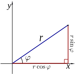
Converting between polar and Cartesian coordinates

A diagram illustrating the relationship between polar and Cartesian coordinates.

The polar coordinates r and φ can be converted to the Cartesian coordinates x and y by using the trigonometric functions sine and cosine:

$${\displaystyle {\begin{aligned}x&=r\cos \varphi ,\\y&=r\sin \varphi .\end{aligned}}}$$

The Cartesian coordinates x and y can be converted to polar coordinates r and φ with r ≥ 0 and φ in the interval (−π, π] by: ^[13]

$${\displaystyle {\begin{aligned}r&={\sqrt {x^{2}+y^{2}}}=\operatorname {hypot} (x,y)\\\varphi &=\operatorname {atan2} (y,x),\end{aligned}}}$$

where hypot is the Pythagorean sum and atan2 is a common variation on the arctangent function defined as

$${\displaystyle \operatorname {atan2} (y,x)={\begin{cases}\arctan \left({\frac {y}{x}}\right)&{\mbox{if }}x>0\\\arctan \left({\frac {y}{x}}\right)+\pi &{\mbox{if }}x<0{\mbox{ and }}y\geq 0\\\arctan \left({\frac {y}{x}}\right)-\pi &{\mbox{if }}x<0{\mbox{ and }}y<0\\{\frac {\pi }{2}}&{\mbox{if }}x=0{\mbox{ and }}y>0\\-{\frac {\pi }{2}}&{\mbox{if }}x=0{\mbox{ and }}y<0\\{\text{undefined}}&{\mbox{if }}x=0{\mbox{ and }}y=0.\end{cases}}}$$

If r is calculated first as above, then this formula for φ may be stated more simply using the arccosine function:

$${\displaystyle \varphi ={\begin{cases}\arccos \left({\frac {x}{r}}\right)&{\mbox{if }}y\geq 0{\mbox{ and }}r\neq 0\\-\arccos \left({\frac {x}{r}}\right)&{\mbox{if }}y<0\\{\text{undefined}}&{\mbox{if }}r=0.\end{cases}}}$$

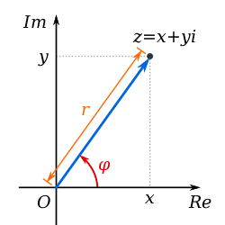
Complex numbers

An illustration of a complex number z plotted on the complex plane

An illustration of a complex number plotted on the complex plane using Euler's formula

Every complex number can be represented as a point in the complex plane, and can therefore be expressed by specifying either the point's Cartesian coordinates (called rectangular or Cartesian form) or the point's polar coordinates (called polar form).

In polar form, the distance and angle coordinates are often referred to as the number's magnitude and argument respectively. Two complex numbers can be multiplied by adding their arguments and multiplying their magnitudes.

The complex number z can be represented in rectangular form as

$${\displaystyle z=x+iy}$$

where i is the imaginary unit, or can alternatively be written in polar form as

$${\displaystyle z=r(\cos \varphi +i\sin \varphi )}$$

and from there, by Euler's formula, ^[14] as

$${\displaystyle z=re^{i\varphi }=r\exp i\varphi .}$$

where e is Euler's number, and φ, expressed in radians, is the principal value of the complex number function arg applied to x + iy. To convert between the rectangular and polar forms of a complex number, the conversion formulae given above can be used. Equivalent are the cis and angle notations:

$${\displaystyle z=r\operatorname {\mathrm {cis} } \varphi =r\angle \varphi .}$$

For the operations of multiplication, division, exponentiation, and root extraction of complex numbers, it is generally much simpler to work with complex numbers expressed in polar form rather than rectangular form. From the laws of exponentiation:

Multiplication

${\displaystyle r_{0}e^{i\varphi _{0}}\,r_{1}e^{i\varphi _{1}}=r_{0}r_{1}e^{i\left(\varphi _{0}+\varphi _{1}\right)}}$

Division

${\displaystyle {\frac {r_{0}e^{i\varphi _{0}}}{r_{1}e^{i\varphi _{1}}}}={\frac {r_{0}}{r_{1}}}e^{i(\varphi _{0}-\varphi _{1})}}$

Exponentiation (De Moivre's formula)

${\displaystyle \left(re^{i\varphi }\right)^{n}=r^{n}e^{in\varphi }}$

Root Extraction (Principal root)

${\displaystyle {\sqrt[{n}]{re^{i\varphi }}}={\sqrt[{n}]{r}}e^{i\varphi \over n}}$

Polar equation of a curve

A curve on the Cartesian plane can be mapped into polar coordinates. In this animation, ${\displaystyle y=\sin(6\!\cdot \!x)+2}$ is mapped onto ${\displaystyle r=\sin(6\!\cdot \!\theta )+2}$. Click on image for details.

The equation defining a plane curve expressed in polar coordinates is known as a polar equation. In many cases, such an equation can simply be specified by defining r as a function of φ. The resulting curve then consists of points of the form (r(φ), φ) and can be regarded as the graph of the polar function r. Note that, in contrast to Cartesian coordinates, the independent variable φ is the second entry in the ordered pair.

Different forms of symmetry can be deduced from the equation of a polar function r:

• If r(−φ) = r(φ) the curve will be symmetrical about the horizontal (0°/180°) ray;
• If r(π − φ) = r(φ) it will be symmetric about the vertical (90°/270°) ray:
• If r(φ − α) = r(φ) it will be rotationally symmetric by α clockwise and counterclockwise about the pole.

Because of the circular nature of the polar coordinate system, many curves can be described by a rather simple polar equation, whereas their Cartesian form is much more intricate. Among the best known of these curves are the polar rose, Archimedean spiral, lemniscate, limaçon, and cardioid.

For the circle, line, and polar rose below, it is understood that there are no restrictions on the domain and range of the curve.

Circle

A circle with equation r(φ) = 1

The general equation for a circle with a center at ${\displaystyle (r_{0},\gamma )}$ and radius a is

$${\displaystyle r^{2}-2rr_{0}\cos(\varphi -\gamma )+r_{0}^{2}=a^{2}.}$$

This can be simplified in various ways, to conform to more specific cases, such as the equation

$${\displaystyle r(\varphi )=a}$$

for a circle with a center at the pole and radius a. ^[15]

When r₀ = a or the origin lies on the circle, the equation becomes

$${\displaystyle r=2a\cos(\varphi -\gamma ).}$$

In the general case, the equation can be solved for r, giving

$${\displaystyle r=r_{0}\cos(\varphi -\gamma )+{\sqrt {a^{2}-r_{0}^{2}\sin ^{2}(\varphi -\gamma )}}}$$

The solution with a minus sign in front of the square root gives the same curve.

Line

Radial lines (those running through the pole) are represented by the equation

$${\displaystyle \varphi =\gamma ,}$$

where ${\displaystyle \gamma }$ is the angle of elevation of the line; that is, ${\displaystyle \varphi =\arctan m}$, where ${\displaystyle m}$ is the slope of the line in the Cartesian coordinate system. The non-radial line that crosses the radial line ${\displaystyle \varphi =\gamma }$ perpendicularly at the point ${\displaystyle (r_{0},\gamma )}$ has the equation

$${\displaystyle r(\varphi )=r_{0}\sec(\varphi -\gamma ).}$$

Otherwise stated ${\displaystyle (r_{0},\gamma )}$ is the point in which the tangent intersects the imaginary circle of radius ${\displaystyle r_{0}}$

Polar rose

A polar rose with equation r(φ) = 2 sin 4φ

A polar rose is a mathematical curve that looks like a petaled flower, and that can be expressed as a simple polar equation,

$${\displaystyle r(\varphi )=a\cos \left(k\varphi +\gamma _{0}\right)}$$

for any constant γ₀ (including 0). If k is an integer, these equations will produce a k-petaled rose if k is odd, or a 2k-petaled rose if k is even. If k is rational, but not an integer, a rose-like shape may form but with overlapping petals. Note that these equations never define a rose with 2, 6, 10, 14, etc. petals. The variable a directly represents the length or amplitude of the petals of the rose, while k relates to their spatial frequency. The constant γ₀ can be regarded as a phase angle.

Archimedean spiral

One arm of an Archimedean spiral with equation r(φ) = φ / 2π for 0 < φ < 6πpi

The Archimedean spiral is a spiral discovered by Archimedes which can also be expressed as a simple polar equation. It is represented by the equation

$${\displaystyle r(\varphi )=a+b\varphi .}$$

Changing the parameter a will turn the spiral, while b controls the distance between the arms, which for a given spiral is always constant. The Archimedean spiral has two arms, one for φ > 0 and one for φ < 0. The two arms are smoothly connected at the pole. If a = 0, taking the mirror image of one arm across the 90°/270° line will yield the other arm. This curve is notable as one of the first curves, after the conic sections, to be described in a mathematical treatise, and as a prime example of a curve best defined by a polar equation.

Ellipse, showing semi-latus rectum

Conic sections

A conic section with one focus on the pole and the other somewhere on the 0° ray (so that the conic's major axis lies along the polar axis) is given by:

$${\displaystyle r={\ell \over {1-e\cos \varphi }}}$$

where e is the eccentricity and ${\displaystyle \ell }$ is the semi-latus rectum (the perpendicular distance at a focus from the major axis to the curve). If e > 1, this equation defines a hyperbola; if e = 1, it defines a parabola; and if e < 1, it defines an ellipse. The special case e = 0 of the latter results in a circle of the radius ${\displaystyle \ell }$.

Intersection of two polar curves

The graphs of two polar functions ${\displaystyle r=f(\theta )}$ and ${\displaystyle r=g(\theta )}$ have possible intersections of three types:

1. In the origin, if the equations ${\displaystyle f(\theta )=0}$ and ${\displaystyle g(\theta )=0}$ have at least one solution each.
2. All the points ${\displaystyle [g(\theta _{i}),\theta _{i}]}$ where ${\displaystyle \theta _{i}}$ are solutions to the equation ${\displaystyle f(\theta +2k\pi )=g(\theta )}$ where ${\displaystyle k}$ is an integer.
3. All the points ${\displaystyle [g(\theta _{i}),\theta _{i}]}$ where ${\displaystyle \theta _{i}}$ are solutions to the equation ${\displaystyle f(\theta +(2k+1)\pi )=-g(\theta )}$ where ${\displaystyle k}$ is an integer.

Calculus

Calculus can be applied to equations expressed in polar coordinates. ^{[16] [17]}

The angular coordinate φ is expressed in radians throughout this section, which is the conventional choice when doing calculus.

Differential calculus

Using x = r cos φ and y = r sin φ, one can derive a relationship between derivatives in Cartesian and polar coordinates. For a given function, u(x,y), it follows that (by computing its total derivatives) or

$${\displaystyle {\begin{aligned}r{\frac {du}{dr}}&=r{\frac {\partial u}{\partial x}}\cos \varphi +r{\frac {\partial u}{\partial y}}\sin \varphi =x{\frac {\partial u}{\partial x}}+y{\frac {\partial u}{\partial y}},\\[2pt]{\frac {du}{d\varphi }}&=-{\frac {\partial u}{\partial x}}r\sin \varphi +{\frac {\partial u}{\partial y}}r\cos \varphi =-y{\frac {\partial u}{\partial x}}+x{\frac {\partial u}{\partial y}}.\end{aligned}}}$$

Hence, we have the following formulae:

$${\displaystyle {\begin{aligned}r{\frac {d}{dr}}&=x{\frac {\partial }{\partial x}}+y{\frac {\partial }{\partial y}}\\[2pt]{\frac {d}{d\varphi }}&=-y{\frac {\partial }{\partial x}}+x{\frac {\partial }{\partial y}}.\end{aligned}}}$$

Using the inverse coordinates transformation, an analogous reciprocal relationship can be derived between the derivatives. Given a function u(r,φ), it follows that

$${\displaystyle {\begin{aligned}{\frac {du}{dx}}&={\frac {\partial u}{\partial r}}{\frac {\partial r}{\partial x}}+{\frac {\partial u}{\partial \varphi }}{\frac {\partial \varphi }{\partial x}},\\[2pt]{\frac {du}{dy}}&={\frac {\partial u}{\partial r}}{\frac {\partial r}{\partial y}}+{\frac {\partial u}{\partial \varphi }}{\frac {\partial \varphi }{\partial y}},\end{aligned}}}$$

or

$${\displaystyle {\begin{aligned}{\frac {du}{dx}}&={\frac {\partial u}{\partial r}}{\frac {x}{\sqrt {x^{2}+y^{2}}}}-{\frac {\partial u}{\partial \varphi }}{\frac {y}{x^{2}+y^{2}}}\\[2pt]&=\cos \varphi {\frac {\partial u}{\partial r}}-{\frac {1}{r}}\sin \varphi {\frac {\partial u}{\partial \varphi }},\\[2pt]{\frac {du}{dy}}&={\frac {\partial u}{\partial r}}{\frac {y}{\sqrt {x^{2}+y^{2}}}}+{\frac {\partial u}{\partial \varphi }}{\frac {x}{x^{2}+y^{2}}}\\[2pt]&=\sin \varphi {\frac {\partial u}{\partial r}}+{\frac {1}{r}}\cos \varphi {\frac {\partial u}{\partial \varphi }}.\end{aligned}}}$$

Hence, we have the following formulae:

$${\displaystyle {\begin{aligned}{\frac {d}{dx}}&=\cos \varphi {\frac {\partial }{\partial r}}-{\frac {1}{r}}\sin \varphi {\frac {\partial }{\partial \varphi }}\\[2pt]{\frac {d}{dy}}&=\sin \varphi {\frac {\partial }{\partial r}}+{\frac {1}{r}}\cos \varphi {\frac {\partial }{\partial \varphi }}.\end{aligned}}}$$

To find the Cartesian slope of the tangent line to a polar curve r(φ) at any given point, the curve is first expressed as a system of parametric equations.

$${\displaystyle {\begin{aligned}x&=r(\varphi )\cos \varphi \\y&=r(\varphi )\sin \varphi \end{aligned}}}$$

Differentiating both equations with respect to φ yields

$${\displaystyle {\begin{aligned}{\frac {dx}{d\varphi }}&=r'(\varphi )\cos \varphi -r(\varphi )\sin \varphi \\[2pt]{\frac {dy}{d\varphi }}&=r'(\varphi )\sin \varphi +r(\varphi )\cos \varphi .\end{aligned}}}$$

Dividing the second equation by the first yields the Cartesian slope of the tangent line to the curve at the point (r(φ), φ):

$${\displaystyle {\frac {dy}{dx}}={\frac {r'(\varphi )\sin \varphi +r(\varphi )\cos \varphi }{r'(\varphi )\cos \varphi -r(\varphi )\sin \varphi }}.}$$

For other useful formulas including divergence, gradient, and Laplacian in polar coordinates, see curvilinear coordinates.

Integral calculus (arc length)

The arc length (length of a line segment) defined by a polar function is found by the integration over the curve r(φ). Let L denote this length along the curve starting from points A through to point B, where these points correspond to φ = a and φ = b such that 0 < b − a < 2π. The length of L is given by the following integral

$${\displaystyle L=\int _{a}^{b}{\sqrt {\left[r(\varphi )\right]^{2}+\left[{\tfrac {dr(\varphi )}{d\varphi }}\right]^{2}}}d\varphi }$$

Integral calculus (area)

The integration region R is bounded by the curve r(φ) and the rays φ = a and φ = b.

Let R denote the region enclosed by a curve r(φ) and the rays φ = a and φ = b, where 0 < b − a ≤ 2π. Then, the area of R is

$${\displaystyle {\frac {1}{2}}\int _{a}^{b}\left[r(\varphi )\right]^{2}\,d\varphi .}$$

The region R is approximated by n sectors (here, n = 5).

A planimeter, which mechanically computes polar integrals

This result can be found as follows. First, the interval [a, b] is divided into n subintervals, where n is some positive integer. Thus Δφ, the angle measure of each subinterval, is equal to b − a (the total angle measure of the interval), divided by n, the number of subintervals. For each subinterval i = 1, 2, ..., n, let φ_i be the midpoint of the subinterval, and construct a sector with the center at the pole, radius r(φ_i), central angle Δφ and arc length r(φ_i)Δφ. The area of each constructed sector is therefore equal to

$${\displaystyle \left[r(\varphi _{i})\right]^{2}\pi \cdot {\frac {\Delta \varphi }{2\pi }}={\frac {1}{2}}\left[r(\varphi _{i})\right]^{2}\Delta \varphi .}$$

Hence, the total area of all of the sectors is

$${\displaystyle \sum _{i=1}^{n}{\tfrac {1}{2}}r(\varphi _{i})^{2}\,\Delta \varphi .}$$

As the number of subintervals n is increased, the approximation of the area improves. Taking n → ∞, the sum becomes the Riemann sum for the above integral.

A mechanical device that computes area integrals is the planimeter, which measures the area of plane figures by tracing them out: this replicates integration in polar coordinates by adding a joint so that the 2-element linkage effects Green's theorem, converting the quadratic polar integral to a linear integral.

Generalization

Using Cartesian coordinates, an infinitesimal area element can be calculated as dA = dxdy. The substitution rule for multiple integrals states that, when using other coordinates, the Jacobian determinant of the coordinate conversion formula has to be considered:

$${\displaystyle J=\det {\frac {\partial (x,y)}{\partial (r,\varphi )}}={\begin{vmatrix}{\frac {\partial x}{\partial r}}&{\frac {\partial x}{\partial \varphi }}\\[2pt]{\frac {\partial y}{\partial r}}&{\frac {\partial y}{\partial \varphi }}\end{vmatrix}}={\begin{vmatrix}\cos \varphi &-r\sin \varphi \\\sin \varphi &r\cos \varphi \end{vmatrix}}=r\cos ^{2}\varphi +r\sin ^{2}\varphi =r.}$$

Hence, an area element in polar coordinates can be written as

$${\displaystyle dA=dx\,dy\ =J\,dr\,d\varphi =r\,dr\,d\varphi .}$$

Now, a function, that is given in polar coordinates, can be integrated as follows:

$${\displaystyle \iint _{R}f(x,y)\,dA=\int _{a}^{b}\int _{0}^{r(\varphi )}f(r,\varphi )\,r\,dr\,d\varphi .}$$

Here, R is the same region as above, namely, the region enclosed by a curve r(φ) and the rays φ = a and φ = b. The formula for the area of R is retrieved by taking f identically equal to 1.

A graph of ${\displaystyle f(x)=e^{-x^{2}}}$ and the area between the function and the ${\displaystyle x}$-axis, which is equal to ${\displaystyle {\sqrt {\pi }}}$.

A more surprising application of this result yields the Gaussian integral:

$${\displaystyle \int _{-\infty }^{\infty }e^{-x^{2}}\,dx={\sqrt {\pi }}.}$$

Vector calculus

Vector calculus can also be applied to polar coordinates. For a planar motion, let ${\displaystyle \mathbf {r} }$ be the position vector (r cos(φ), r sin(φ)), with r and φ depending on time t.

We define an orthonormal basis with three unit vectors: radial, transverse, and normal directions. The radial direction is defined by normalizing ${\displaystyle \mathbf {r} }$:

$${\displaystyle {\hat {\mathbf {r} }}=(\cos(\varphi ),\sin(\varphi ))}$$

Radial and velocity directions span the plane of the motion, whose normal direction is denoted ${\displaystyle {\hat {\mathbf {k} }}}$:

$${\displaystyle {\hat {\mathbf {k} }}={\hat {\mathbf {v} }}\times {\hat {\mathbf {r} }}.}$$

The transverse direction is perpendicular to both radial and normal directions:

$${\displaystyle {\hat {\boldsymbol {\varphi }}}=(-\sin(\varphi ),\cos(\varphi ))={\hat {\mathbf {k} }}\times {\hat {\mathbf {r} }}\ ,}$$

Then

$${\displaystyle {\begin{aligned}\mathbf {r} &=(x,\ y)=r(\cos \varphi ,\ \sin \varphi )=r{\hat {\mathbf {r} }}\ ,\\{\dot {\mathbf {r} }}&=\left({\dot {x}},\ {\dot {y}}\right)={\dot {r}}(\cos \varphi ,\ \sin \varphi )+r{\dot {\varphi }}(-\sin \varphi ,\ \cos \varphi )={\dot {r}}{\hat {\mathbf {r} }}+r{\dot {\varphi }}{\hat {\boldsymbol {\varphi }}}\ ,\\{\ddot {\mathbf {r} }}&=\left({\ddot {x}},\ {\ddot {y}}\right)\\&={\ddot {r}}(\cos \varphi ,\ \sin \varphi )+2{\dot {r}}{\dot {\varphi }}(-\sin \varphi ,\ \cos \varphi )+r{\ddot {\varphi }}(-\sin \varphi ,\ \cos \varphi )-r{\dot {\varphi }}^{2}(\cos \varphi ,\ \sin \varphi )\\&=\left({\ddot {r}}-r{\dot {\varphi }}^{2}\right){\hat {\mathbf {r} }}+\left(r{\ddot {\varphi }}+2{\dot {r}}{\dot {\varphi }}\right){\hat {\boldsymbol {\varphi }}}\\&=\left({\ddot {r}}-r{\dot {\varphi }}^{2}\right){\hat {\mathbf {r} }}+{\frac {1}{r}}\;{\frac {d}{dt}}\left(r^{2}{\dot {\varphi }}\right){\hat {\boldsymbol {\varphi }}}.\end{aligned}}}$$

This equation can be obtain by taking derivative of the function and derivatives of the unit basis vectors.

For a curve in 2D where the parameter is ${\displaystyle \theta }$ the previous equations simplify to:

$${\displaystyle {\begin{aligned}{\vec {r}}&=r(\theta ){\hat {e}}_{r}\\{\frac {d{\vec {r}}}{d\theta }}&={\frac {dr}{d\theta }}{\hat {e}}_{r}+r{\hat {e}}_{\theta }\\{\frac {d^{2}{\vec {r}}}{d\theta ^{2}}}&=\left({\frac {d^{2}r}{d\theta ^{2}}}-r\right){\hat {e}}_{r}+{\frac {dr}{d\theta }}{\hat {e}}_{\theta }\end{aligned}}}$$

Centrifugal and Coriolis terms

See also: Mechanics of planar particle motion and Centrifugal force (rotating reference frame)

Position vector r, always points radially from the origin.

Velocity vector v, always tangent to the path of motion.

Acceleration vector a, not parallel to the radial motion but offset by the angular and Coriolis accelerations, nor tangent to the path but offset by the centripetal and radial accelerations.

Kinematic vectors in plane polar coordinates. Notice the setup is not restricted to 2d space, but a plane in any higher dimension.

The term ${\displaystyle r{\dot {\varphi }}^{2}}$ is sometimes referred to as the centripetal acceleration, and the term ${\displaystyle 2{\dot {r}}{\dot {\varphi }}}$ as the Coriolis acceleration. For example, see Shankar. ^[18]

Note: these terms, that appear when acceleration is expressed in polar coordinates, are a mathematical consequence of differentiation; they appear whenever polar coordinates are used. In planar particle dynamics these accelerations appear when setting up Newton's second law of motion in a rotating frame of reference. Here these extra terms are often called fictitious forces; fictitious because they are simply a result of a change in coordinate frame. That does not mean they do not exist, rather they exist only in the rotating frame.

Inertial frame of reference S and instantaneous non-inertial co-rotating frame of reference S′. The co-rotating frame rotates at angular rate Ω equal to the rate of rotation of the particle about the origin of S′ at the particular moment t. Particle is located at vector position r(t) and unit vectors are shown in the radial direction to the particle from the origin, and also in the direction of increasing angle ϕ normal to the radial direction. These unit vectors need not be related to the tangent and normal to the path. Also, the radial distance r need not be related to the radius of curvature of the path.

Co-rotating frame

For a particle in planar motion, one approach to attaching physical significance to these terms is based on the concept of an instantaneous co-rotating frame of reference. ^[19] To define a co-rotating frame, first an origin is selected from which the distance r(t) to the particle is defined. An axis of rotation is set up that is perpendicular to the plane of motion of the particle, and passing through this origin. Then, at the selected moment t, the rate of rotation of the co-rotating frame Ω is made to match the rate of rotation of the particle about this axis, dφ/dt. Next, the terms in the acceleration in the inertial frame are related to those in the co-rotating frame. Let the location of the particle in the inertial frame be (r(t), φ(t)), and in the co-rotating frame be (r′(t), φ′(t)). Because the co-rotating frame rotates at the same rate as the particle, dφ′/dt = 0. The fictitious centrifugal force in the co-rotating frame is mrΩ², radially outward. The velocity of the particle in the co-rotating frame also is radially outward, because dφ′/dt = 0. The fictitious Coriolis force therefore has a value −2m(dr/dt)Ω, pointed in the direction of increasing φ only. Thus, using these forces in Newton's second law we find:

$${\displaystyle {\boldsymbol {F}}+{\boldsymbol {F}}_{\text{cf}}+{\boldsymbol {F}}_{\text{Cor}}=m{\ddot {\boldsymbol {r}}}\ ,}$$

where over dots represent time differentiations, and F is the net real force (as opposed to the fictitious forces). In terms of components, this vector equation becomes:

$${\displaystyle {\begin{aligned}F_{r}+mr\Omega ^{2}&=m{\ddot {r}}\\F_{\varphi }-2m{\dot {r}}\Omega &=mr{\ddot {\varphi }}\ ,\end{aligned}}}$$

which can be compared to the equations for the inertial frame:

$${\displaystyle {\begin{aligned}F_{r}&=m{\ddot {r}}-mr{\dot {\varphi }}^{2}\\F_{\varphi }&=mr{\ddot {\varphi }}+2m{\dot {r}}{\dot {\varphi }}\ .\end{aligned}}}$$

This comparison, plus the recognition that by the definition of the co-rotating frame at time t it has a rate of rotation Ω = dφ/dt, shows that we can interpret the terms in the acceleration (multiplied by the mass of the particle) as found in the inertial frame as the negative of the centrifugal and Coriolis forces that would be seen in the instantaneous, non-inertial co-rotating frame.

For general motion of a particle (as opposed to simple circular motion), the centrifugal and Coriolis forces in a particle's frame of reference commonly are referred to the instantaneous osculating circle of its motion, not to a fixed center of polar coordinates. For more detail, see centripetal force.

Differential geometry

In the modern terminology of differential geometry, polar coordinates provide coordinate charts for the differentiable manifold R² \ {(0,0)}, the plane minus the origin. In these coordinates, the Euclidean metric tensor is given by

$${\displaystyle ds^{2}=dr^{2}+r^{2}d\theta ^{2}.}$$

This can be seen via the change of variables formula for the metric tensor, or by computing the differential forms dx, dy via the exterior derivative of the 0-forms x = r cos(θ), y = r sin(θ) and substituting them in the Euclidean metric tensor ds² = dx² + dy². An orthonormal frame with respect to this metric is given by

$${\displaystyle e_{r}={\frac {\partial }{\partial r}},\quad e_{\theta }={\frac {1}{r}}{\frac {\partial }{\partial \theta }},}$$

with dual coframe

$${\displaystyle e^{r}=dr,\quad e^{\theta }=rd\theta .}$$

The connection form relative to this frame and the Levi-Civita connection is given by the skew-symmetric matrix of 1-forms

$${\displaystyle {\omega ^{i}}_{j}={\begin{pmatrix}0&-d\theta \\d\theta &0\end{pmatrix}}}$$

and hence the curvature form Ω = dω + ω∧ω vanishes. Therefore, as expected, the punctured plane is a flat manifold.

Extensions in 3D

The polar coordinate system is extended into three dimensions with two different coordinate systems, the cylindrical and spherical coordinate system.

Applications

Polar coordinates are two-dimensional and thus they can be used only where point positions lie on a single two-dimensional plane. They are most appropriate in any context where the phenomenon being considered is inherently tied to direction and length from a center point. For instance, the examples above show how elementary polar equations suffice to define curves—such as the Archimedean spiral—whose equation in the Cartesian coordinate system would be much more intricate. Moreover, many physical systems—such as those concerned with bodies moving around a central point or with phenomena originating from a central point—are simpler and more intuitive to model using polar coordinates. The initial motivation for the introduction of the polar system was the study of circular and orbital motion.

Position and navigation

Polar coordinates are used often in navigation as the destination or direction of travel can be given as an angle and distance from the object being considered. For instance, aircraft use a slightly modified version of the polar coordinates for navigation. In this system, the one generally used for any sort of navigation, the 0° ray is generally called heading 360, and the angles continue in a clockwise direction, rather than counterclockwise, as in the mathematical system. Heading 360 corresponds to magnetic north, while headings 90, 180, and 270 correspond to magnetic east, south, and west, respectively. ^[20] Thus, an aircraft traveling 5 nautical miles due east will be traveling 5 units at heading 90 (read zero-niner-zero by air traffic control). ^[21]

Modeling

Systems displaying radial symmetry provide natural settings for the polar coordinate system, with the central point acting as the pole. A prime example of this usage is the groundwater flow equation when applied to radially symmetric wells. Systems with a radial force are also good candidates for the use of the polar coordinate system. These systems include gravitational fields, which obey the inverse-square law, as well as systems with point sources, such as radio antennas.

Radially asymmetric systems may also be modeled with polar coordinates. For example, a microphone's pickup pattern illustrates its proportional response to an incoming sound from a given direction, and these patterns can be represented as polar curves. The curve for a standard cardioid microphone, the most common unidirectional microphone, can be represented as r = 0.5 + 0.5sin(ϕ) at its target design frequency. ^[22] The pattern shifts toward omnidirectionality at lower frequencies.

See also

• Mathematics portal

• Curvilinear coordinates
• List of canonical coordinate transformations
• Log-polar coordinates
• Polar decomposition
• Unit circle

References

1. Brown, Richard G. (1997). Andrew M. Gleason (ed.). Advanced Mathematics: Precalculus with Discrete Mathematics and Data Analysis. Evanston, Illinois: McDougal Littell. ISBN   0-395-77114-5.
2. Friendly, Michael (August 24, 2009). "Milestones in the History of Thematic Cartography, Statistical Graphics, and Data Visualization" (PDF). Archived from the original (PDF) on September 26, 2018. Retrieved July 23, 2016.
3. King, David A. (2005). "The Sacred Geography of Islam". In Koetsier, Teun; Luc, Bergmans (eds.). Mathematics and the Divine: A Historical Study. Amsterdam: Elsevier. pp. 162–78. ISBN   0-444-50328-5.
4. King (2005, p. 169). The calculations were as accurate as could be achieved under the limitations imposed by their assumption that the Earth was a perfect sphere.
5. Coolidge, Julian (1952). "The Origin of Polar Coordinates". American Mathematical Monthly. 59 (2). Mathematical Association of America: 78–85. doi:10.2307/2307104. JSTOR   2307104.
6. Boyer, C. B. (1949). "Newton as an Originator of Polar Coordinates". American Mathematical Monthly. 56 (2). Mathematical Association of America: 73–78. doi:10.2307/2306162. JSTOR   2306162.
7. Miller, Jeff. "Earliest Known Uses of Some of the Words of Mathematics" . Retrieved 2006-09-10.
8. Smith, David Eugene (1925). History of Mathematics, Vol II. Boston: Ginn and Co. p. 324.
9. Serway, Raymond A.; Jewett Jr., John W. (2005). Principles of Physics. Brooks/Cole—Thomson Learning. ISBN   0-534-49143-X.
10. "Polar Coordinates and Graphing" (PDF). 2006-04-13. Archived from the original (PDF) on August 22, 2016. Retrieved 2006-09-22.
11. Lee, Theodore; David Cohen; David Sklar (2005). Precalculus: With Unit-Circle Trigonometry (Fourth ed.). Thomson Brooks/Cole. ISBN   0-534-40230-5.
12. Stewart, Ian; David Tall (1983). Complex Analysis (the Hitchhiker's Guide to the Plane). Cambridge University Press. ISBN   0-521-28763-4.
13. Torrence, Bruce Follett; Eve Torrence (1999). The Student's Introduction to Mathematica. Cambridge University Press. ISBN   0-521-59461-8.
14. Smith, Julius O. (2003). "Euler's Identity". Mathematics of the Discrete Fourier Transform (DFT). W3K Publishing. ISBN   0-9745607-0-7. Archived from the original on 2006-09-15. Retrieved 2006-09-22.
15. Claeys, Johan. "Polar coordinates". Archived from the original on 2006-04-27. Retrieved 2006-05-25.
16. Husch, Lawrence S. "Areas Bounded by Polar Curves". Archived from the original on 2000-03-01. Retrieved 2006-11-25.
17. Lawrence S. Husch. "Tangent Lines to Polar Graphs". Archived from the original on 2019-11-21. Retrieved 2006-11-25.
18. Ramamurti Shankar (1994). Principles of Quantum Mechanics (2nd ed.). Springer. p. 81. ISBN   0-306-44790-8.
19. For the following discussion, see John R Taylor (2005). Classical Mechanics. University Science Books. p. §9.10, pp. 358–359. ISBN   1-891389-22-X.
20. Santhi, Sumrit. "Aircraft Navigation System" . Retrieved 2006-11-26.
21. "Emergency Procedures" (PDF). Archived from the original (PDF) on 2013-06-03. Retrieved 2007-01-15.
22. Eargle, John (2005). Handbook of Recording Engineering (Fourth ed.). Springer. ISBN   0-387-28470-2.

General references

• Adams, Robert; Christopher Essex (2013). Calculus: a complete course (Eighth ed.). Pearson Canada Inc. ISBN   978-0-321-78107-9.
• Anton, Howard; Irl Bivens; Stephen Davis (2002). Calculus (Seventh ed.). Anton Textbooks, Inc. ISBN   0-471-38157-8.
• Finney, Ross; George Thomas; Franklin Demana; Bert Waits (June 1994). Calculus: Graphical, Numerical, Algebraic (Single Variable Version ed.). Addison-Wesley Publishing Co. ISBN   0-201-55478-X.

External links

• "Polar coordinates", Encyclopedia of Mathematics , EMS Press, 2001 [1994]
• Graphing Software at Curlie
• Coordinate Converter — converts between polar, Cartesian and spherical coordinates
• Polar Coordinate System Dynamic Demo