Related rates

Last updated

In differential calculus, related rates problems involve finding a rate at which a quantity changes by relating that quantity to other quantities whose rates of change are known. The rate of change is usually with respect to time. Because science and engineering often relate quantities to each other, the methods of related rates have broad applications in these fields. Differentiation with respect to time or one of the other variables requires application of the chain rule, [1] since most problems involve several variables.

Contents

Fundamentally, if a function is defined such that , then the derivative of the function can be taken with respect to another variable. We assume is a function of , i.e. . Then , so

Written in Leibniz notation, this is:

Thus, if it is known how changes with respect to , then we can determine how changes with respect to and vice versa. We can extend this application of the chain rule with the sum, difference, product and quotient rules of calculus, etc.

For example, if then

Procedure

The most common way to approach related rates problems is the following: [2]

  1. Identify the known variables, including rates of change and the rate of change that is to be found. (Drawing a picture or representation of the problem can help to keep everything in order)
  2. Construct an equation relating the quantities whose rates of change are known to the quantity whose rate of change is to be found.
  3. Differentiate both sides of the equation with respect to time (or other rate of change). Often, the chain rule is employed at this step.
  4. Substitute the known rates of change and the known quantities into the equation.
  5. Solve for the wanted rate of change.

Errors in this procedure are often caused by plugging in the known values for the variables before (rather than after) finding the derivative with respect to time. Doing so will yield an incorrect result, since if those values are substituted for the variables before differentiation, those variables will become constants; and when the equation is differentiated, zeroes appear in places of all variables for which the values were plugged in.

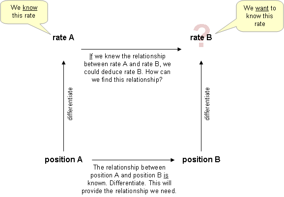
FourCorner RelatedRates.png

Example

A 10-meter ladder is leaning against the wall of a building, and the base of the ladder is sliding away from the building at a rate of 3 meters per second. How fast is the top of the ladder sliding down the wall when the base of the ladder is 6 meters from the wall?

The distance between the base of the ladder and the wall, x, and the height of the ladder on the wall, y, represent the sides of a right triangle with the ladder as the hypotenuse, h. The objective is to find dy/dt, the rate of change of y with respect to time, t, when h, x and dx/dt, the rate of change of x, are known.

Step 1:

Step 2: From the Pythagorean theorem, the equation

describes the relationship between x, y and h, for a right triangle. Differentiating both sides of this equation with respect to time, t, yields

Step 3: When solved for the wanted rate of change, dy/dt, gives us

Step 4 & 5: Using the variables from step 1 gives us:

Solving for y using the Pythagorean Theorem gives:

Plugging in 8 for the equation:

It is generally assumed that negative values represent the downward direction. In doing such, the top of the ladder is sliding down the wall at a rate of 9/4 meters per second.

Physics examples

Because one physical quantity often depends on another, which, in turn depends on others, such as time, related-rates methods have broad applications in Physics. This section presents an example of related rates kinematics and electromagnetic induction.

Relative kinematics of two vehicles

One vehicle is headed North and currently located at (0,3); the other vehicle is headed West and currently located at (4,0). The chain rule can be used to find whether they are getting closer or further apart. Physics intersection.png
One vehicle is headed North and currently located at (0,3); the other vehicle is headed West and currently located at (4,0). The chain rule can be used to find whether they are getting closer or further apart.

For example, one can consider the kinematics problem where one vehicle is heading West toward an intersection at 80 miles per hour while another is heading North away from the intersection at 60 miles per hour. One can ask whether the vehicles are getting closer or further apart and at what rate at the moment when the North bound vehicle is 3 miles North of the intersection and the West bound vehicle is 4 miles East of the intersection.

Big idea: use chain rule to compute rate of change of distance between two vehicles.

Plan:

  1. Choose coordinate system
  2. Identify variables
  3. Draw picture
  4. Big idea: use chain rule to compute rate of change of distance between two vehicles
  5. Express c in terms of x and y via Pythagorean theorem
  6. Express dc/dt using chain rule in terms of dx/dt and dy/dt
  7. Substitute in x, y, dx/dt, dy/dt
  8. Simplify.

Choose coordinate system: Let the y-axis point North and the x-axis point East.

Identify variables: Define y(t) to be the distance of the vehicle heading North from the origin and x(t) to be the distance of the vehicle heading West from the origin.

Expresscin terms ofx and yvia the Pythagorean theorem:

Expressdc/dtusing chain rule in terms ofdx/dtanddy/dt:

Apply derivative operator to entire function
Square root is outside function; Sum of squares is inside function
Distribute differentiation operator
Apply chain rule to x(t) and y(t)}
Simplify.

Substitute inx = 4 mi, y = 3 mi, dx/dt = −80 mi/hr, dy/dt = 60 mi/hr and simplify

Consequently, the two vehicles are getting closer together at a rate of 28 mi/hr.

Electromagnetic induction of conducting loop spinning in magnetic field

The magnetic flux through a loop of area A whose normal is at an angle θ to a magnetic field of strength B is

Faraday's law of electromagnetic induction states that the induced electromotive force is the negative rate of change of magnetic flux through a conducting loop.

If the loop area A and magnetic field B are held constant, but the loop is rotated so that the angle θ is a known function of time, the rate of change of θ can be related to the rate of change of (and therefore the electromotive force) by taking the time derivative of the flux relation

If for example, the loop is rotating at a constant angular velocity ω, so that θ = ωt, then

Related Research Articles

In calculus, the chain rule is a formula that expresses the derivative of the composition of two differentiable functions f and g in terms of the derivatives of f and g. More precisely, if is the function such that for every x, then the chain rule is, in Lagrange's notation,
<span class="mw-page-title-main">Equations of motion</span> Equations that describe the behavior of a physical system

In physics, equations of motion are equations that describe the behavior of a physical system in terms of its motion as a function of time. More specifically, the equations of motion describe the behavior of a physical system as a set of mathematical functions in terms of dynamic variables. These variables are usually spatial coordinates and time, but may include momentum components. The most general choice are generalized coordinates which can be any convenient variables characteristic of the physical system. The functions are defined in a Euclidean space in classical mechanics, but are replaced by curved spaces in relativity. If the dynamics of a system is known, the equations are the solutions for the differential equations describing the motion of the dynamics.

The calculus of variations is a field of mathematical analysis that uses variations, which are small changes in functions and functionals, to find maxima and minima of functionals: mappings from a set of functions to the real numbers. Functionals are often expressed as definite integrals involving functions and their derivatives. Functions that maximize or minimize functionals may be found using the Euler–Lagrange equation of the calculus of variations.

In mathematics, an implicit equation is a relation of the form where R is a function of several variables. For example, the implicit equation of the unit circle is

<span class="mw-page-title-main">Separation of variables</span> Technique for solving differential equations

In mathematics, separation of variables is any of several methods for solving ordinary and partial differential equations, in which algebra allows one to rewrite an equation so that each of two variables occurs on a different side of the equation.

In mathematics, especially vector calculus and differential topology, a closed form is a differential form α whose exterior derivative is zero, and an exact form is a differential form, α, that is the exterior derivative of another differential form β. Thus, an exact form is in the image of d, and a closed form is in the kernel of d.

A continuity equation or transport equation is an equation that describes the transport of some quantity. It is particularly simple and powerful when applied to a conserved quantity, but it can be generalized to apply to any extensive quantity. Since mass, energy, momentum, electric charge and other natural quantities are conserved under their respective appropriate conditions, a variety of physical phenomena may be described using continuity equations.

In mathematics, the total derivative of a function f at a point is the best linear approximation near this point of the function with respect to its arguments. Unlike partial derivatives, the total derivative approximates the function with respect to all of its arguments, not just a single one. In many situations, this is the same as considering all partial derivatives simultaneously. The term "total derivative" is primarily used when f is a function of several variables, because when f is a function of a single variable, the total derivative is the same as the ordinary derivative of the function.

In mathematical analysis, and applications in geometry, applied mathematics, engineering, and natural sciences, a function of a real variable is a function whose domain is the real numbers , or a subset of that contains an interval of positive length. Most real functions that are considered and studied are differentiable in some interval. The most widely considered such functions are the real functions, which are the real-valued functions of a real variable, that is, the functions of a real variable whose codomain is the set of real numbers.

A time derivative is a derivative of a function with respect to time, usually interpreted as the rate of change of the value of the function. The variable denoting time is usually written as .

In calculus, a parametric derivative is a derivative of a dependent variable with respect to another dependent variable that is taken when both variables depend on an independent third variable, usually thought of as "time".

In mathematics, a change of variables is a basic technique used to simplify problems in which the original variables are replaced with functions of other variables. The intent is that when expressed in new variables, the problem may become simpler, or equivalent to a better understood problem.

In calculus, the Leibniz integral rule for differentiation under the integral sign, named after Gottfried Leibniz, states that for an integral of the form

<span class="mw-page-title-main">Multiple integral</span> Generalization of definite integrals to functions of multiple variables

In mathematics, a multiple integral is a definite integral of a function of several real variables, for instance, f(x, y) or f(x, y, z). Integrals of a function of two variables over a region in are called double integrals, and integrals of a function of three variables over a region in are called triple integrals. For multiple integrals of a single-variable function, see the Cauchy formula for repeated integration.

<span class="mw-page-title-main">Second derivative</span> Mathematical operation

In calculus, the second derivative, or the second order derivative, of a function f is the derivative of the derivative of f. Roughly speaking, the second derivative measures how the rate of change of a quantity is itself changing; for example, the second derivative of the position of an object with respect to time is the instantaneous acceleration of the object, or the rate at which the velocity of the object is changing with respect to time. In Leibniz notation:

<span class="mw-page-title-main">Hopf bifurcation</span> Critical point where a periodic solution arises

In the mathematical theory of bifurcations, a Hopfbifurcation is a critical point where a system's stability switches and a periodic solution arises. More accurately, it is a local bifurcation in which a fixed point of a dynamical system loses stability, as a pair of complex conjugate eigenvalues—of the linearization around the fixed point—crosses the complex plane imaginary axis. Under reasonably generic assumptions about the dynamical system, a small-amplitude limit cycle branches from the fixed point.

In differential calculus, there is no single uniform notation for differentiation. Instead, various notations for the derivative of a function or variable have been proposed by various mathematicians. The usefulness of each notation varies with the context, and it is sometimes advantageous to use more than one notation in a given context. The most common notations for differentiation are listed below.

<span class="mw-page-title-main">Differentiation of trigonometric functions</span> Mathematical process of finding the derivative of a trigonometric function

The differentiation of trigonometric functions is the mathematical process of finding the derivative of a trigonometric function, or its rate of change with respect to a variable. For example, the derivative of the sine function is written sin′(a) = cos(a), meaning that the rate of change of sin(x) at a particular angle x = a is given by the cosine of that angle.

The Cauchy momentum equation is a vector partial differential equation put forth by Cauchy that describes the non-relativistic momentum transport in any continuum.

In calculus, the differential represents the principal part of the change in a function y = f(x) with respect to changes in the independent variable. The differential dy is defined by

References

  1. "Related Rates". Whitman College. Retrieved 2013-10-27.
  2. Kreider, Donald. "Related Rates". Dartmouth. Retrieved 2013-10-27.