This article needs additional citations for verification .(December 2020) |
In finance, the beta (β or market beta or beta coefficient) is a statistic that measures the expected increase or decrease of an individual stock price in proportion to movements of the stock market as a whole. Beta can be used to indicate the contribution of an individual asset to the market risk of a portfolio when it is added in small quantity. It refers to an asset's non-diversifiable risk, systematic risk, or market risk. Beta is not a measure of idiosyncratic risk.
Beta is the hedge ratio of an investment with respect to the stock market. For example, to hedge out the market-risk of a stock with a market beta of 2.0, an investor would short $2,000 in the stock market for every $1,000 invested in the stock. Thus insured, movements of the overall stock market no longer influence the combined position on average. Beta measures the contribution of an individual investment to the risk of the market portfolio that was not reduced by diversification. It does not measure the risk when an investment is held on a stand-alone basis.
The beta of an asset is compared to the market as a whole, usually the S&P 500. By definition, the value-weighted average of all market-betas of all investable assets with respect to the value-weighted market index is 1. If an asset has a beta above 1, it indicates that its return moves more than 1-to-1 with the return of the market-portfolio, on average; that is, it is more volatile than the market. In practice, few stocks have negative betas (tending to go up when the market goes down). Most stocks have betas between 0 and 3. [1]
Most fixed income instruments and commodities tend to have low or zero betas; call options tend to have high betas; and put options and short positions and some inverse ETFs tend to have negative betas.
The market beta of an asset , observed on occasions, is defined by (and best obtained via) a linear regression of the rate of return of asset on the rate of return of the (typically value-weighted) stock-market index :
where is an unbiased error term whose squared error should be minimized. The coefficient is often referred to as the alpha.
The ordinary least squares solution is:
where and are the covariance and variance operators. Betas with respect to different market indexes are not comparable.
By using the relationship between standard deviation and variance, and the definition of correlation , market beta can also be written as
where is the correlation of the two returns, and , are the respective volatilities. This equation shows that the idiosyncratic risk () is related to but often very different to market beta. If the idiosyncratic risk is 0 (i.e., the stock returns do not move), so is the market-beta. The reverse is not the case: A coin toss bet has a zero beta but not zero risk.
Attempts have been made to estimate the three ingredient components separately, but this has not led to better estimates of market-betas.
Suppose an investor has all his money in the market and wishes to move a small amount into asset class . The new portfolio is defined by
The variance can be computed as
For small values of , the terms in can be ignored,
Using the definition of this is
This suggests that an asset with greater than 1 increases the portfolio variance, while an asset with less than 1 decreases it if added in a small amount.
Market-beta can be weighted, averaged, added, etc. That is, if a portfolio consists of 80% asset A and 20% asset B, then the beta of the portfolio is 80% times the beta of asset A and 20% times the beta of asset B.
![]() | This section possibly contains original research .(December 2020) |
In practice, the choice of index makes relatively little difference in the market betas of individual assets, because broad value-weighted market indexes tend to move closely together. Academics tend to prefer to work with a value-weighted market portfolio due to its attractive aggregation properties and its close link with the capital asset pricing model (CAPM). [2] Practitioners tend to prefer to work with the S&P 500 due to its easy in-time availability and availability to hedge with stock index futures.
In the idealized CAPM, beta risk is the only kind of risk for which investors should receive an expected return higher than the risk-free rate of interest. [3] When used within the context of the CAPM, beta becomes a measure of the appropriate expected rate of return. Due to the fact that the overall rate of return on the firm is weighted rate of return on its debt and its equity, the market-beta of the overall unlevered firm is the weighted average of the firm's debt beta (often close to 0) and its levered equity beta.
In fund management, adjusting for exposure to the market separates out the component that fund managers should have received given that they had their specific exposure to the market. For example, if the stock market went up by 20% in a given year, and a manager had a portfolio with a market-beta of 2.0, this portfolio should have returned 40% in the absence of specific stock picking skills. This is measured by the alpha in the market-model, holding beta constant.
Occasionally, other betas than market-betas are used. The arbitrage pricing theory (APT) has multiple factors in its model and thus requires multiple betas. (The CAPM has only one risk factor, namely the overall market, and thus works only with the plain beta.) For example, a beta with respect to oil price changes would sometimes be called an "oil-beta" rather than "market-beta" to clarify the difference.
Betas commonly quoted in mutual fund analyses often measure the exposure to a specific fund benchmark, rather than to the overall stock market. Such a beta would measure the risk from adding a specific fund to a holder of the mutual fund benchmark portfolio, rather than the risk of adding the fund to a portfolio of the market. [4]
Utility stocks commonly show up as examples of low beta. These have some similarity to bonds, in that they tend to pay consistent dividends, and their prospects are not strongly dependent on economic cycles. They are still stocks, so the market price will be affected by overall stock market trends, even if this does not make sense.
Foreign stocks may provide some diversification. World benchmarks such as S&P Global 100 have slightly lower betas than comparable US-only benchmarks such as S&P 100. However, this effect is not as good as it used to be; the various markets are now fairly correlated, especially the US and Western Europe.[ citation needed ]
Derivatives are examples of non-linear assets. Whereas Beta relies on a linear model, an out of the money option will have a distinctly non-linear payoff. In these cases, then, the change in price of an option relative to the change in the price of its underlying asset is not constant. (True also - but here, far less pronounced - for volatility, time to expiration, and other factors.) Thus "beta" here, calculated traditionally, would vary constantly as the price of the underlying changed.
Accommodating this, mathematical finance defines a specific volatility beta. [5] Here, analogous to the above, this beta represents the covariance between the derivative's return and changes in the value of the underlying asset, with, additionally, a correction for instantaneous underlying changes. See volatility (finance), volatility risk, Greeks (finance) § Vega.
A true beta (which defines the true expected relationship between the rate of return on assets and the market) differs from a realized beta that is based on historical rates of returns and represents just one specific history out of the set of possible stock return realizations. The true market-beta is essentially the average outcome if infinitely many draws could be observed. On average, the best forecast of the realized market-beta is also the best forecast of the true market-beta.
Estimators of market-beta have to wrestle with two important problems. First, the underlying market betas are known to move over time. Second, investors are interested in the best forecast of the true prevailing beta most indicative of the most likely future beta realization and not in the historical market-beta.
Despite these problems, a historical beta estimator remains an obvious benchmark predictor. It is obtained as the slope of the fitted line from the linear least-squares estimator. The OLS regression can be estimated on 1–5 years worth of daily, weekly or monthly stock returns. The choice depends on the trade off between accuracy of beta measurement (longer periodic measurement times and more years give more accurate results) and historic firm beta changes over time (for example, due to changing sales products or clients).
Other beta estimators reflect the tendency of betas (like rates of return) for regression toward the mean, induced not only by measurement error but also by underlying changes in the true beta and/or historical randomness. (Intuitively, one would not suggest a company with high return [e.g., a drug discovery] last year also to have as high a return next year.) Such estimators include the Blume/Bloomberg beta [6] (used prominently on many financial websites), the Vasicek beta, [7] the Scholes–Williams beta, [8] the Dimson beta, [9] and the Welch beta. [10]
These estimators attempt to uncover the instant prevailing market-beta. When long-term market-betas are required, further regression toward the mean over long horizons should be considered.
In finance, the capital asset pricing model (CAPM) is a model used to determine a theoretically appropriate required rate of return of an asset, to make decisions about adding assets to a well-diversified portfolio.
In statistics, the Gauss–Markov theorem states that the ordinary least squares (OLS) estimator has the lowest sampling variance within the class of linear unbiased estimators, if the errors in the linear regression model are uncorrelated, have equal variances and expectation value of zero. The errors do not need to be normal, nor do they need to be independent and identically distributed. The requirement that the estimator be unbiased cannot be dropped, since biased estimators exist with lower variance. See, for example, the James–Stein estimator, ridge regression, or simply any degenerate estimator.
In mathematical finance, the Greeks are the quantities representing the sensitivity of the price of a derivative instrument such as an option to changes in one or more underlying parameters on which the value of an instrument or portfolio of financial instruments is dependent. The name is used because the most common of these sensitivities are denoted by Greek letters. Collectively these have also been called the risk sensitivities, risk measures or hedge parameters.
Modern portfolio theory (MPT), or mean-variance analysis, is a mathematical framework for assembling a portfolio of assets such that the expected return is maximized for a given level of risk. It is a formalization and extension of diversification in investing, the idea that owning different kinds of financial assets is less risky than owning only one type. Its key insight is that an asset's risk and return should not be assessed by itself, but by how it contributes to a portfolio's overall risk and return. The variance of return is used as a measure of risk, because it is tractable when assets are combined into portfolios. Often, the historical variance and covariance of returns is used as a proxy for the forward-looking versions of these quantities, but other, more sophisticated methods are available.
In finance, arbitrage pricing theory (APT) is a multi-factor model for asset pricing which relates various macro-economic (systematic) risk variables to the pricing of financial assets. Proposed by economist Stephen Ross in 1976, it is widely believed to be an improved alternative to its predecessor, the capital asset pricing model (CAPM). APT is founded upon the law of one price, which suggests that within an equilibrium market, rational investors will implement arbitrage such that the equilibrium price is eventually realised. As such, APT argues that when opportunities for arbitrage are exhausted in a given period, then the expected return of an asset is a linear function of various factors or theoretical market indices, where sensitivities of each factor is represented by a factor-specific beta coefficient or factor loading. Consequently, it provides traders with an indication of ‘true’ asset value and enables exploitation of market discrepancies via arbitrage. The linear factor model structure of the APT is used as the basis for evaluating asset allocation, the performance of managed funds as well as the calculation of cost of capital. Furthermore, the newer APT model is more dynamic being utilised in more theoretical application than the preceding CAPM model. A 1986 article written by Gregory Connor and Robert Korajczyk, utilised the APT framework and applied it to portfolio performance measurement suggesting that the Jensen coefficient is an acceptable measurement of portfolio performance.
In finance, the duration of a financial asset that consists of fixed cash flows, such as a bond, is the weighted average of the times until those fixed cash flows are received. When the price of an asset is considered as a function of yield, duration also measures the price sensitivity to yield, the rate of change of price with respect to yield, or the percentage change in price for a parallel shift in yields.
In finance, Jensen's alpha is used to determine the abnormal return of a security or portfolio of securities over the theoretical expected return. It is a version of the standard alpha based on a theoretical performance instead of a market index.
In statistics, econometrics, epidemiology and related disciplines, the method of instrumental variables (IV) is used to estimate causal relationships when controlled experiments are not feasible or when a treatment is not successfully delivered to every unit in a randomized experiment. Intuitively, IVs are used when an explanatory variable of interest is correlated with the error term (endogenous), in which case ordinary least squares and ANOVA give biased results. A valid instrument induces changes in the explanatory variable but has no independent effect on the dependent variable and is not correlated with the error term, allowing a researcher to uncover the causal effect of the explanatory variable on the dependent variable.
In statistics, ordinary least squares (OLS) is a type of linear least squares method for choosing the unknown parameters in a linear regression model by the principle of least squares: minimizing the sum of the squares of the differences between the observed dependent variable in the input dataset and the output of the (linear) function of the independent variable. Some sources consider OLS to be linear regression.
In statistics, simple linear regression (SLR) is a linear regression model with a single explanatory variable. That is, it concerns two-dimensional sample points with one independent variable and one dependent variable and finds a linear function that, as accurately as possible, predicts the dependent variable values as a function of the independent variable. The adjective simple refers to the fact that the outcome variable is related to a single predictor.
In statistics, the delta method is a method of deriving the asymptotic distribution of a random variable. It is applicable when the random variable being considered can be defined as a differentiable function of a random variable which is asymptotically Gaussian.
In statistics, generalized least squares (GLS) is a method used to estimate the unknown parameters in a linear regression model. It is used when there is a non-zero amount of correlation between the residuals in the regression model. GLS is employed to improve statistical efficiency and reduce the risk of drawing erroneous inferences, as compared to conventional least squares and weighted least squares methods. It was first described by Alexander Aitken in 1935.
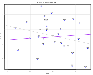
Security market line (SML) is the representation of the capital asset pricing model. It displays the expected rate of return of an individual security as a function of systematic, non-diversifiable risk. The risk of an individual risky security reflects the volatility of the return from the security rather than the return of the market portfolio. The risk in these individual risky securities reflects the systematic risk.
The single-index model (SIM) is a simple asset pricing model to measure both the risk and the return of a stock. The model has been developed by William Sharpe in 1963 and is commonly used in the finance industry. Mathematically the SIM is expressed as:
Fixed-income attribution is the process of measuring returns generated by various sources of risk in a fixed income portfolio, particularly when multiple sources of return are active at the same time.
In corporate finance, Hamada’s equation is an equation used as a way to separate the financial risk of a levered firm from its business risk. The equation combines the Modigliani–Miller theorem with the capital asset pricing model. It is used to help determine the levered beta and, through this, the optimal capital structure of firms. It was named after Robert Hamada, the Professor of Finance behind the theory.
In statistics, principal component regression (PCR) is a regression analysis technique that is based on principal component analysis (PCA). More specifically, PCR is used for estimating the unknown regression coefficients in a standard linear regression model.
In investing, downside beta is the beta that measures a stock's association with the overall stock market (risk) only on days when the market’s return is negative. Downside beta was first proposed by Roy 1952 and then popularized in an investment book by Markowitz (1959).
In investing, upside beta is the element of traditional beta that investors do not typically associate with the true meaning of risk. It is defined to be the scaled amount by which an asset tends to move compared to a benchmark, calculated only on days when the benchmark's return is positive.
Untradable assets are assets that are not traded on the market. Human capital is the most important nontraded assets. Other important nontraded asset classes are private businesses, claims to government transfer payments and claims on trust income.