Arbitrage pricing theory

Last updated

In finance, arbitrage pricing theory (APT) is a multi-factor model for asset pricing which relates various macro-economic (systematic) risk variables to the pricing of financial assets. Proposed by economist Stephen Ross in 1976, [1] it is widely believed to be an improved alternative to its predecessor, the Capital Asset Pricing Model (CAPM). [2] APT is founded upon the law of one price, which suggests that within an equilibrium market, rational investors will implement arbitrage such that the equilibrium price is eventually realised. [2] As such, APT argues that when opportunities for arbitrage are exhausted in a given period, then the expected return of an asset is a linear function of various factors or theoretical market indices, where sensitivities of each factor is represented by a factor-specific beta coefficient or factor loading. Consequently, it provides traders with an indication of ‘true’ asset value and enables exploitation of market discrepancies via arbitrage. The linear factor model structure of the APT is used as the basis for evaluating asset allocation, the performance of managed funds as well as the calculation of cost of capital. [3] Furthermore, the newer APT model is more dynamic being utilised in more theoretical application than the preceding CAPM model. A 1986 article written by Gregory Connor and Robert Korajczyk, utilised the APT framework and applied it to portfolio performance measurement suggesting that the Jensen coefficient is an acceptable measurement of portfolio performance. [4]

Contents

Model

APT is a single-period static model, which helps investors understand the trade-off between risk and return. The average investor aims to optimise the returns for any given level or risk and as such, expects a positive return for bearing greater risk. As per the APT model, risky asset returns are said to follow a factor intensity structure if they can be expressed as:

where
  • is a constant for asset
  • is a systematic factor
  • is the sensitivity of the th asset to factor , also called factor loading,
  • and is the risky asset's idiosyncratic random shock with mean zero.

Idiosyncratic shocks are assumed to be uncorrelated across assets and uncorrelated with the factors.

The APT model states that if asset returns follow a factor structure then the following relation exists between expected returns and the factor sensitivities:

where

That is, the expected return of an asset j is a linear function of the asset's sensitivities to the n factors.

Note that there are some assumptions and requirements that have to be fulfilled for the latter to be correct: There must be perfect competition in the market, and the total number of factors may never surpass the total number of assets (in order to avoid the problem of matrix singularity).

General Model

For a set of assets with returns , factor loadings , and factors , a general factor model that is used in APT is:

where follows a multivariate normal distribution. In general, it is useful to assume that the factors are distributed as:

where is the expected risk premium vector and is the factor covariance matrix. Assuming that the noise terms for the returns and factors are uncorrelated, the mean and covariance for the returns are respectively:

It is generally assumed that we know the factors in a model, which allows least squares to be utilized. However, an alternative to this is to assume that the factors are latent variables and employ factor analysis - akin to the form used in psychometrics - to extract them.

Assumptions of APT Model

The APT model for asset valuation is founded on the following assumptions: [2]

  1. Investors are risk-averse in nature and possess the same expectations
  2. Efficient markets with limited opportunity for arbitrage
  3. Perfect capital markets
  4. Infinite number of assets
  5. Risk factors are indicative of systematic risks that cannot be diversified away and thus impact all financial assets, to some degree. Thus, these factors must be:    
    • Non-specific to any individual firm or industry
    • Compensated by the market via a risk premium
    • A random variable

Arbitrage

Arbitrage is the practice whereby investors take advantage of slight variations in asset valuation from its fair price, to generate a profit. It is the realisation of a positive expected return from overvalued or undervalued securities in the inefficient market without any incremental risk and zero additional investments.

Mechanics

In the APT context, arbitrage consists of trading in two assets with at least one being mispriced. The arbitrageur sells the asset which is relatively too expensive and uses the proceeds to buy one which is relatively too cheap.

Under the APT, an asset is mispriced if its current price diverges from the price predicted by the model. The asset price today should equal the sum of all future cash flows discounted at the APT rate, where the expected return of the asset is a linear function of various factors, and sensitivity to changes in each factor is represented by a factor-specific beta coefficient.

A correctly priced asset here may be in fact a synthetic asset - a portfolio consisting of other correctly priced assets. This portfolio has the same exposure to each of the macroeconomic factors as the mispriced asset. The arbitrageur creates the portfolio by identifying n correctly priced assets (one per risk-factor, plus one) and then weighting the assets such that portfolio beta per factor is the same as for the mispriced asset.

When the investor is long the asset and short the portfolio (or vice versa) he has created a position which has a positive expected return (the difference between asset return and portfolio return) and which has a net zero exposure to any macroeconomic factor and is therefore risk free (other than for firm specific risk). The arbitrageur is thus in a position to make a risk-free profit:

Where today's price is too low:

The implication is that at the end of the period the portfolio would have appreciated at the rate implied by the APT, whereas the mispriced asset would have appreciated at more than this rate. The arbitrageur could therefore:
Today:
1 short sell the portfolio
2 buy the mispriced asset with the proceeds.
At the end of the period:
1 sell the mispriced asset
2 use the proceeds to buy back the portfolio
3 pocket the difference.

Where today's price is too high:

The implication is that at the end of the period the portfolio would have appreciated at the rate implied by the APT, whereas the mispriced asset would have appreciated at less than this rate. The arbitrageur could therefore:
Today:
1 short sell the mispriced asset
2 buy the portfolio with the proceeds.
At the end of the period:
1 sell the portfolio
2 use the proceeds to buy back the mispriced asset
3 pocket the difference.

Difference between the capital asset pricing model

The APT along with the capital asset pricing model (CAPM) is one of two influential theories on asset pricing. The APT differs from the CAPM in that it is less restrictive in its assumptions, making it more flexible for use in a wider range of application. Thus, it possesses greator explanatory power (as opposed to statistical) for expected asset returns. It assumes that each investor will hold a unique portfolio with its own particular array of betas, as opposed to the identical "market portfolio". In some ways, the CAPM can be considered a "special case" of the APT in that the securities market line represents a single-factor model of the asset price, where beta is exposed to changes in value of the market.

Fundamentally, the CAPM is derived on the premise that all factors in the economy can be reconciled into one factor represented by a market portfolio, thus implying they all have equivalent weight on the asset’s return. In contrast, the APT model suggests that each stock reacts uniquely to various macroeconomic factors and thus the impact of each must be accounted for separately. [2]

A disadvantage of APT is that the selection and the number of factors to use in the model is ambiguous. Most academics use three to five factors to model returns, but the factors selected have not been empirically robust. In many instances the CAPM, as a model to estimate expected returns, has empirically outperformed the more advanced APT. [5]

Additionally, the APT can be seen as a "supply-side" model, since its beta coefficients reflect the sensitivity of the underlying asset to economic factors. Thus, factor shocks would cause structural changes in assets' expected returns, or in the case of stocks, in firms' profitabilities.

On the other side, the capital asset pricing model is considered a "demand side" model. Its results, although similar to those of the APT, arise from a maximization problem of each investor's utility function, and from the resulting market equilibrium (investors are considered to be the "consumers" of the assets).

Implementation

As with the CAPM, the factor-specific betas are found via a linear regression of historical security returns on the factor in question. Unlike the CAPM, the APT, however, does not itself reveal the identity of its priced factors - the number and nature of these factors is likely to change over time and between economies. As a result, this issue is essentially empirical in nature. Several a priori guidelines as to the characteristics required of potential factors are, however, suggested:

  1. their impact on asset prices manifests in their unexpected movements and they are completely unpredictable to the market at the beginning of each period [2]
  2. they should represent undiversifiable influences (these are, clearly, more likely to be macroeconomic rather than firm-specific in nature) on expected returns and so must be quantifiable with non-zero prices [2]
  3. timely and accurate information on these variables is required
  4. the relationship should be theoretically justifiable on economic grounds

Chen, Roll and Ross identified the following macro-economic factors as significant in explaining security returns: [6]

As a practical matter, indices or spot or futures market prices may be used in place of macro-economic factors, which are reported at low frequency (e.g. monthly) and often with significant estimation errors. Market indices are sometimes derived by means of factor analysis. More direct "indices" that might be used are:

International Arbitrage Pricing Theory

International Arbitrage pricing theory (IAPT) is an important extension of the base idea of arbitrage pricing theory which further considers factors such as exchange rate risk. In 1983 Bruno Solnik created an extension of the original arbitrage pricing theory to include risk related to international exchange rates hence making the model applicable international markets with multi-currency transactions. Solnik suggested that there may be several factors common to all international assets, and conversely, there may be other common factors applicable to certain markets based on nationality. [7]

Fama and French originally proposed a three-factor model in 1995 which, consistent with the suggestion from Solnik above suggests that integrated international markets may experience a common set of factors, hence making it possible to price assets in all integrated markets using their model. The Fama and French three factor model attempts to explain stock returns based on market risk, size, and value. [8]

A 2012 paper aimed to empirically investigate Solnik’s IAPT model and the suggestion that base currency fluctuations have a direct and comprehendible effect on the risk premiums of assets. This was tested by generating a returns relation which broke down individual investor returns into currency and non-currency (universal) returns. The paper utilised Fama and French’s three factor model (explained above) to estimate international currency impacts on common factors. It was concluded that the total foreign exchange risk in international markets consisted of the immediate exchange rate risk and the residual market factors. This, along with empirical data tests validates the idea that foreign currency fluctuations have a direct effect on risk premiums and the factor loadings included in the APT model, hence, confirming the validity of the IAPT model. [9]

See also

Related Research Articles

Financial economics is the branch of economics characterized by a "concentration on monetary activities", in which "money of one type or another is likely to appear on both sides of a trade". Its concern is thus the interrelation of financial variables, such as share prices, interest rates and exchange rates, as opposed to those concerning the real economy. It has two main areas of focus: asset pricing and corporate finance; the first being the perspective of providers of capital, i.e. investors, and the second of users of capital. It thus provides the theoretical underpinning for much of finance.

<span class="mw-page-title-main">Capital asset pricing model</span> Model used in finance

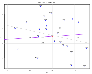
In finance, the capital asset pricing model (CAPM) is a model used to determine a theoretically appropriate required rate of return of an asset, to make decisions about adding assets to a well-diversified portfolio.

<span class="mw-page-title-main">Efficient-market hypothesis</span> Economic theory that asset prices fully reflect all available information

The efficient-market hypothesis (EMH) is a hypothesis in financial economics that states that asset prices reflect all available information. A direct implication is that it is impossible to "beat the market" consistently on a risk-adjusted basis since market prices should only react to new information.

Rational pricing is the assumption in financial economics that asset prices – and hence asset pricing models – will reflect the arbitrage-free price of the asset as any deviation from this price will be "arbitraged away". This assumption is useful in pricing fixed income securities, particularly bonds, and is fundamental to the pricing of derivative instruments.

Modern portfolio theory (MPT), or mean-variance analysis, is a mathematical framework for assembling a portfolio of assets such that the expected return is maximized for a given level of risk. It is a formalization and extension of diversification in investing, the idea that owning different kinds of financial assets is less risky than owning only one type. Its key insight is that an asset's risk and return should not be assessed by itself, but by how it contributes to a portfolio's overall risk and return. It uses the past variance of asset prices as a proxy for future risk.

In finance, the beta is a statistic that measures the expected increase or decrease of an individual stock price in proportion to movements of the Stock market as a whole. Beta can be used to indicate the contribution of an individual asset to the market risk of a portfolio when it is added in small quantity. It is referred to as an asset's non-diversifiable risk, systematic risk, or market risk. Beta is not a measure of idiosyncratic risk.

In finance, Jensen's alpha is used to determine the abnormal return of a security or portfolio of securities over the theoretical expected return. It is a version of the standard alpha based on a theoretical performance instead of a market index.

Alpha is a measure of the active return on an investment, the performance of that investment compared with a suitable market index. An alpha of 1% means the investment's return on investment over a selected period of time was 1% better than the market during that same period; a negative alpha means the investment underperformed the market. Alpha, along with beta, is one of two key coefficients in the capital asset pricing model used in modern portfolio theory and is closely related to other important quantities such as standard deviation, R-squared and the Sharpe ratio.

A market anomaly in a financial market is predictability that seems to be inconsistent with theories of asset prices. Standard theories include the capital asset pricing model and the Fama-French Three Factor Model, but a lack of agreement among academics about the proper theory leads many to refer to anomalies without a reference to a benchmark theory. Indeed, many academics simply refer to anomalies as "return predictors", avoiding the problem of defining a benchmark theory.

The following outline is provided as an overview of and topical guide to finance:

The single-index model (SIM) is a simple asset pricing model to measure both the risk and the return of a stock. The model has been developed by William Sharpe in 1963 and is commonly used in the finance industry. Mathematically the SIM is expressed as:

The consumption-based capital asset pricing model (CCAPM) is a model of the determination of expected return on an investment. The foundations of this concept were laid by the research of Robert Lucas (1978) and Douglas Breeden (1979).

Roll's critique is a famous analysis of the validity of empirical tests of the capital asset pricing model (CAPM) by Richard Roll. It concerns methods to formally test the statement of the CAPM, the equation

In asset pricing and portfolio management the Fama–French three-factor model is a statistical model designed in 1992 by Eugene Fama and Kenneth French to describe stock returns. Fama and French were colleagues at the University of Chicago Booth School of Business, where Fama still works. In 2013, Fama shared the Nobel Memorial Prize in Economic Sciences for his empirical analysis of asset prices. The three factors are (1) market excess return, (2) the outperformance of small versus big companies, and (3) the outperformance of high book/market versus low book/market companies. There is academic debate about the last two factors.

A portfolio manager (PM) is a professional responsible for making investment decisions and carrying out investment activities on behalf of vested individuals or institutions. Clients invest their money into the PM's investment policy for future growth, such as a retirement fund, endowment fund, or education fund. PMs work with a team of analysts and researchers and are responsible for establishing an investment strategy, selecting appropriate investments, and allocating each investment properly towards an investment fund or asset management vehicle.

In Finance the Treynor–Black model is a mathematical model for security selection published by Fischer Black and Jack Treynor in 1973. The model assumes an investor who considers that most securities are priced efficiently, but who believes they have information that can be used to predict the abnormal performance (Alpha) of a few of them; the model finds the optimum portfolio to hold under such conditions.

<span class="mw-page-title-main">Low-volatility anomaly</span>

In investing and finance, the low-volatility anomaly is the observation that low-volatility stocks have higher returns than high-volatility stocks in most markets studied. This is an example of a stock market anomaly since it contradicts the central prediction of many financial theories that taking higher risk must be compensated with higher returns.

Returns-based style analysis is a statistical technique used in finance to deconstruct the returns of investment strategies using a variety of explanatory variables. The model results in a strategy's exposures to asset classes or other factors, interpreted as a measure of a fund or portfolio manager's investment style. While the model is most frequently used to show an equity mutual fund’s style with reference to common style axes, recent applications have extended the model’s utility to model more complex strategies, such as those employed by hedge funds.

In portfolio management, the Carhart four-factor model is an extra factor addition in the Fama–French three-factor model, proposed by Mark Carhart. The Fama-French model, developed in the 1990, argued most stock market returns are explained by three factors: risk, price and company size. Carhart added a momentum factor for asset pricing of stocks. The Four Factor Model is also known in the industry as the Monthly Momentum Factor (MOM). Momentum is the speed or velocity of price changes in a stock, security, or tradable instrument.

Nontraded assets are assets that are not traded on the market. Human capital is the most important nontraded assets. Other important nontraded asset classes are private businesses, claims to government transfer payments and claims on trust income.

References

  1. Ross, Stephen A (1976-12-01). "The arbitrage theory of capital asset pricing". Journal of Economic Theory. 13 (3): 341–360. doi:10.1016/0022-0531(76)90046-6. ISSN   0022-0531.
  2. 1 2 3 4 5 6 Basu, Debarati; Chawla, Deepak (2012). "An Empirical Test of the Arbitrage Pricing Theory—The Case of Indian Stock Market". Global Business Review. 13 (3): 421–432. doi:10.1177/097215091201300305. ISSN   0972-1509. S2CID   154470693.
  3. Huberman, G. & Wang, Z. (2005). "Arbitrage Pricing Theory" (PDF).{{cite web}}: CS1 maint: multiple names: authors list (link)
  4. Connor, Gregory; Korajczyk, Robert (1986). "Performance measurement with the arbitrage pricing theory: A new framework for analysis". Journal of Financial Economics. 15 (3): 373–394. doi:10.1016/0304-405X(86)90027-9. S2CID   54620410.
  5. French, Jordan (1 March 2017). "Macroeconomic Forces and Arbitrage Pricing Theory". Journal of Comparative Asian Development. 16 (1): 1–20. doi:10.1080/15339114.2017.1297245. S2CID   157510462.
  6. Chen, Nai-Fu; Roll, Richard; Ross, Stephen A. (1986). "Economic Forces and the Stock Market". The Journal of Business. 59 (3): 383–403. doi:10.1086/296344. ISSN   0021-9398. JSTOR   2352710.
  7. Solnik, Bruno (1983). "International Arbitrage Pricing Theory". The Journal of Finance. 38 (2): 449–457. doi:10.2307/2327978. JSTOR   2327978.
  8. Fama, Eugene; French, Kenneth (1996). "Multifactor Explanations of Asset Pricing Anomalies". The Journal of Finance. 51 (1): 55–84. doi:10.1111/j.1540-6261.1996.tb05202.x.
  9. Armstrong, Will; Knif, Johan; Kolari, James; Pynnonen, Seppo (2012). "Exchange risk and universal returns:A test of international arbitrage pricing theory". Pacific Basin Finance Journal. 20 (1): 24–40. doi:10.1016/j.pacfin.2011.08.003.

Further reading