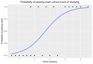
In statistics, the logistic model is a statistical model that models the log-odds of an event as a linear combination of one or more independent variables. In regression analysis, logistic regression estimates the parameters of a logistic model. In binary logistic regression there is a single binary dependent variable, coded by an indicator variable, where the two values are labeled "0" and "1", while the independent variables can each be a binary variable or a continuous variable. The corresponding probability of the value labeled "1" can vary between 0 and 1, hence the labeling; the function that converts log-odds to probability is the logistic function, hence the name. The unit of measurement for the log-odds scale is called a logit, from logistic unit, hence the alternative names. See § Background and § Definition for formal mathematics, and § Example for a worked example.

In statistical modeling, regression analysis is a set of statistical processes for estimating the relationships between a dependent variable and one or more error-free independent variables. The most common form of regression analysis is linear regression, in which one finds the line that most closely fits the data according to a specific mathematical criterion. For example, the method of ordinary least squares computes the unique line that minimizes the sum of squared differences between the true data and that line. For specific mathematical reasons, this allows the researcher to estimate the conditional expectation of the dependent variable when the independent variables take on a given set of values. Less common forms of regression use slightly different procedures to estimate alternative location parameters or estimate the conditional expectation across a broader collection of non-linear models.
The general linear model or general multivariate regression model is a compact way of simultaneously writing several multiple linear regression models. In that sense it is not a separate statistical linear model. The various multiple linear regression models may be compactly written as
In statistics, the coefficient of multiple correlation is a measure of how well a given variable can be predicted using a linear function of a set of other variables. It is the correlation between the variable's values and the best predictions that can be computed linearly from the predictive variables.

In statistics, the coefficient of determination, denoted R2 or r2 and pronounced "R squared", is the proportion of the variation in the dependent variable that is predictable from the independent variable(s).
In statistics, econometrics, epidemiology and related disciplines, the method of instrumental variables (IV) is used to estimate causal relationships when controlled experiments are not feasible or when a treatment is not successfully delivered to every unit in a randomized experiment. Intuitively, IVs are used when an explanatory variable of interest is correlated with the error term (endogenous), in which case ordinary least squares and ANOVA give biased results. A valid instrument induces changes in the explanatory variable but has no independent effect on the dependent variable and is not correlated with the error term, allowing a researcher to uncover the causal effect of the explanatory variable on the dependent variable.
In statistics, omitted-variable bias (OVB) occurs when a statistical model leaves out one or more relevant variables. The bias results in the model attributing the effect of the missing variables to those that were included.

In statistics, ordinary least squares (OLS) is a type of linear least squares method for choosing the unknown parameters in a linear regression model by the principle of least squares: minimizing the sum of the squares of the differences between the observed dependent variable in the input dataset and the output of the (linear) function of the independent variable. Some sources consider OLS to be linear regression.

Regression dilution, also known as regression attenuation, is the biasing of the linear regression slope towards zero, caused by errors in the independent variable.
In statistics, the residual sum of squares (RSS), also known as the sum of squared residuals (SSR) or the sum of squared estimate of errors (SSE), is the sum of the squares of residuals. It is a measure of the discrepancy between the data and an estimation model, such as a linear regression. A small RSS indicates a tight fit of the model to the data. It is used as an optimality criterion in parameter selection and model selection.

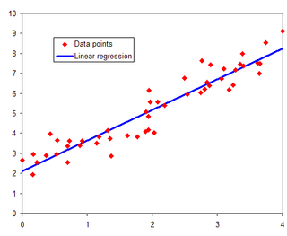
In statistics, simple linear regression (SLR) is a linear regression model with a single explanatory variable. That is, it concerns two-dimensional sample points with one independent variable and one dependent variable and finds a linear function that, as accurately as possible, predicts the dependent variable values as a function of the independent variable. The adjective simple refers to the fact that the outcome variable is related to a single predictor.
Multilevel models are statistical models of parameters that vary at more than one level. An example could be a model of student performance that contains measures for individual students as well as measures for classrooms within which the students are grouped. These models can be seen as generalizations of linear models, although they can also extend to non-linear models. These models became much more popular after sufficient computing power and software became available.

In statistics, a mediation model seeks to identify and explain the mechanism or process that underlies an observed relationship between an independent variable and a dependent variable via the inclusion of a third hypothetical variable, known as a mediator variable. Rather than a direct causal relationship between the independent variable and the dependent variable, which is often false, a mediation model proposes that the independent variable influences the mediator variable, which in turn influences the dependent variable. Thus, the mediator variable serves to clarify the nature of the relationship between the independent and dependent variables.
In statistics, the variance inflation factor (VIF) is the ratio (quotient) of the variance of a parameter estimate when fitting a full model that includes other parameters to the variance of the parameter estimate if the model is fit with only the parameter on its own. The VIF provides an index that measures how much the variance of an estimated regression coefficient is increased because of collinearity.

In statistics, least-angle regression (LARS) is an algorithm for fitting linear regression models to high-dimensional data, developed by Bradley Efron, Trevor Hastie, Iain Johnstone and Robert Tibshirani.
In statistics and regression analysis, moderation occurs when the relationship between two variables depends on a third variable. The third variable is referred to as the moderator variable or simply the moderator. The effect of a moderating variable is characterized statistically as an interaction; that is, a categorical or continuous variable that is associated with the direction and/or magnitude of the relation between dependent and independent variables. Specifically within a correlational analysis framework, a moderator is a third variable that affects the zero-order correlation between two other variables, or the value of the slope of the dependent variable on the independent variable. In analysis of variance (ANOVA) terms, a basic moderator effect can be represented as an interaction between a focal independent variable and a factor that specifies the appropriate conditions for its operation.
In statistics, polynomial regression is a form of regression analysis in which the relationship between the independent variable x and the dependent variable y is modeled as an nth degree polynomial in x. Polynomial regression fits a nonlinear relationship between the value of x and the corresponding conditional mean of y, denoted E(y |x). Although polynomial regression fits a nonlinear model to the data, as a statistical estimation problem it is linear, in the sense that the regression function E(y | x) is linear in the unknown parameters that are estimated from the data. For this reason, polynomial regression is considered to be a special case of multiple linear regression.

Bivariate analysis is one of the simplest forms of quantitative (statistical) analysis. It involves the analysis of two variables, for the purpose of determining the empirical relationship between them.
In statistics and in machine learning, a linear predictor function is a linear function of a set of coefficients and explanatory variables, whose value is used to predict the outcome of a dependent variable. This sort of function usually comes in linear regression, where the coefficients are called regression coefficients. However, they also occur in various types of linear classifiers, as well as in various other models, such as principal component analysis and factor analysis. In many of these models, the coefficients are referred to as "weights".
In statistics, linear regression is a statistical model which estimates the linear relationship between a scalar response and one or more explanatory variables. The case of one explanatory variable is called simple linear regression; for more than one, the process is called multiple linear regression. This term is distinct from multivariate linear regression, where multiple correlated dependent variables are predicted, rather than a single scalar variable. If the explanatory variables are measured with error then errors-in-variables models are required, also known as measurement error models.


