Related Research Articles
In statistics, point estimation involves the use of sample data to calculate a single value which is to serve as a "best guess" or "best estimate" of an unknown population parameter. More formally, it is the application of a point estimator to the data to obtain a point estimate.

In statistics, an expectation–maximization (EM) algorithm is an iterative method to find (local) maximum likelihood or maximum a posteriori (MAP) estimates of parameters in statistical models, where the model depends on unobserved latent variables. The EM iteration alternates between performing an expectation (E) step, which creates a function for the expectation of the log-likelihood evaluated using the current estimate for the parameters, and a maximization (M) step, which computes parameters maximizing the expected log-likelihood found on the E step. These parameter-estimates are then used to determine the distribution of the latent variables in the next E step.

A sensor array is a group of sensors, usually deployed in a certain geometry pattern, used for collecting and processing electromagnetic or acoustic signals. The advantage of using a sensor array over using a single sensor lies in the fact that an array adds new dimensions to the observation, helping to estimate more parameters and improve the estimation performance. For example an array of radio antenna elements used for beamforming can increase antenna gain in the direction of the signal while decreasing the gain in other directions, i.e., increasing signal-to-noise ratio (SNR) by amplifying the signal coherently. Another example of sensor array application is to estimate the direction of arrival of impinging electromagnetic waves. The related processing method is called array signal processing. A third examples includes chemical sensor arrays, which utilize multiple chemical sensors for fingerprint detection in complex mixtures or sensing environments. Application examples of array signal processing include radar/sonar, wireless communications, seismology, machine condition monitoring, astronomical observations fault diagnosis, etc.
This glossary of statistics and probability is a list of definitions of terms and concepts used in the mathematical sciences of statistics and probability, their sub-disciplines, and related fields. For additional related terms, see Glossary of mathematics and Glossary of experimental design.
In time series analysis, the Box–Jenkins method, named after the statisticians George Box and Gwilym Jenkins, applies autoregressive moving average (ARMA) or autoregressive integrated moving average (ARIMA) models to find the best fit of a time-series model to past values of a time series.
In statistics, a generalized additive model (GAM) is a generalized linear model in which the linear response variable depends linearly on unknown smooth functions of some predictor variables, and interest focuses on inference about these smooth functions.
A mixed model, mixed-effects model or mixed error-component model is a statistical model containing both fixed effects and random effects. These models are useful in a wide variety of disciplines in the physical, biological and social sciences. They are particularly useful in settings where repeated measurements are made on the same statistical units, or where measurements are made on clusters of related statistical units. Because of their advantage in dealing with missing values, mixed effects models are often preferred over more traditional approaches such as repeated measures analysis of variance.
In statistics, shrinkage is the reduction in the effects of sampling variation. In regression analysis, a fitted relationship appears to perform less well on a new data set than on the data set used for fitting. In particular the value of the coefficient of determination 'shrinks'. This idea is complementary to overfitting and, separately, to the standard adjustment made in the coefficient of determination to compensate for the subjunctive effects of further sampling, like controlling for the potential of new explanatory terms improving the model by chance: that is, the adjustment formula itself provides "shrinkage." But the adjustment formula yields an artificial shrinkage.
In statistics, confirmatory factor analysis (CFA) is a special form of factor analysis, most commonly used in social science research. It is used to test whether measures of a construct are consistent with a researcher's understanding of the nature of that construct. As such, the objective of confirmatory factor analysis is to test whether the data fit a hypothesized measurement model. This hypothesized model is based on theory and/or previous analytic research. CFA was first developed by Jöreskog (1969) and has built upon and replaced older methods of analyzing construct validity such as the MTMM Matrix as described in Campbell & Fiske (1959).
In statistical signal processing, the goal of spectral density estimation (SDE) or simply spectral estimation is to estimate the spectral density of a signal from a sequence of time samples of the signal. Intuitively speaking, the spectral density characterizes the frequency content of the signal. One purpose of estimating the spectral density is to detect any periodicities in the data, by observing peaks at the frequencies corresponding to these periodicities.
ASReml is a statistical software package for fitting linear mixed models using restricted maximum likelihood, a technique commonly used in plant and animal breeding and quantitative genetics as well as other fields. It is notable for its ability to fit very large and complex data sets efficiently, due to its use of the average information algorithm and sparse matrix methods.
In statistics, quasi-likelihood methods are used to estimate parameters in a statistical model when exact likelihood methods, for example maximum likelihood estimation, are computationally infeasible. Due to the wrong likelihood being used, quasi-likelihood estimators lose asymptotic efficiency compared to, e.g., maximum likelihood estimators. Under broadly applicable conditions, quasi-likelihood estimators are consistent and asymptotically normal. The asymptotic covariance matrix can be obtained using the so-called sandwich estimator. Examples of quasi-likelihood methods include the generalized estimating equations and pairwise likelihood approaches.
In statistics, the method of estimating equations is a way of specifying how the parameters of a statistical model should be estimated. This can be thought of as a generalisation of many classical methods—the method of moments, least squares, and maximum likelihood—as well as some recent methods like M-estimators.
In statistics, a generalized estimating equation (GEE) is used to estimate the parameters of a generalized linear model with a possible unmeasured correlation between observations from different timepoints. Although some believe that Generalized estimating equations are robust in everything even with the wrong choice of working-correlation matrix, Generalized estimating equations are only robust to loss of consistency with the wrong choice.
Shayle Robert Searle PhD was a New Zealand mathematician who was professor emeritus of biological statistics at Cornell University. He was a leader in the field of linear and mixed models in statistics, and published widely on the topics of linear models, mixed models, and variance component estimation.
In statistics Wilks' theorem offers an asymptotic distribution of the log-likelihood ratio statistic, which can be used to produce confidence intervals for maximum-likelihood estimates or as a test statistic for performing the likelihood-ratio test.
Genome-wide complex trait analysis (GCTA) Genome-based restricted maximum likelihood (GREML) is a statistical method for heritability estimation in genetics, which quantifies the total additive contribution of a set of genetic variants to a trait. GCTA is typically applied to common single nucleotide polymorphisms (SNPs) on a genotyping array and thus termed "chip" or "SNP" heritability.
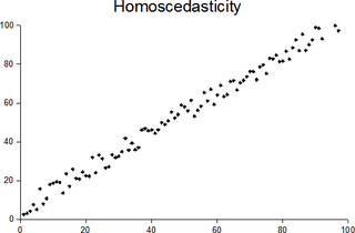
In statistics, a sequence of random variables is homoscedastic if all its random variables have the same finite variance; this is also known as homogeneity of variance. The complementary notion is called heteroscedasticity, also known as heterogeneity of variance. The spellings homoskedasticity and heteroskedasticity are also frequently used. Assuming a variable is homoscedastic when in reality it is heteroscedastic results in unbiased but inefficient point estimates and in biased estimates of standard errors, and may result in overestimating the goodness of fit as measured by the Pearson coefficient.
References
- 1 2 3 Dodge, Yadolah (2006). The Oxford Dictionary of Statistical Terms . Oxford [Oxfordshire]: Oxford University Press. ISBN 0-19-920613-9. (see REML)
- ↑ Baker, Bob. Estimating variances and covariances (broken, original link) available at the Wayback Machine
- ↑ Bartlett, M. S. (1937). "Properties of Sufficiency and Statistical Tests". Proceedings of the Royal Society A: Mathematical, Physical and Engineering Sciences. 160 (901): 268–282. Bibcode:1937RSPSA.160..268B. doi:10.1098/rspa.1937.0109.
- ↑ Patterson, H. D.; Thompson, R. (1971). "Recovery of inter-block information when block sizes are unequal". Biometrika. 58 (3): 545. doi:10.1093/biomet/58.3.545.
- ↑ Harville, D. A. (1977). "Maximum Likelihood Approaches to Variance Component Estimation and to Related Problems". Journal of the American Statistical Association. 72 (358): 320–338. doi:10.2307/2286796. JSTOR 2286796.
- ↑ "Detecting sparse signals in random fields, with an application to brain mapping" (PDF).
- ↑ "SurfStat". www.math.mcgill.ca.
- ↑ "fitlme Documentation". www.mathworks.com.
| | This statistics-related article is a stub. You can help Wikipedia by expanding it. |